PostgreSQL Database

Installation

macOS

Linux/Unix

Step 1: Installing PostgreSQL

# Create the file repository configuration:
sudo sh -c 'echo "deb http://apt.postgresql.org/pub/repos/apt $(lsb_release -cs)-pgdg main" > /etc/apt/sources.list.d/pgdg.list'

# Import the repository signing key:
wget --quiet -O - https://www.postgresql.org/media/keys/ACCC4CF8.asc | sudo apt-key add -

# Update the package lists:
sudo apt-get update

# Install the latest version of PostgreSQL.
# If you want a specific version, use 'postgresql-12' or similar instead of 'postgresql':
sudo apt-get install postgresql

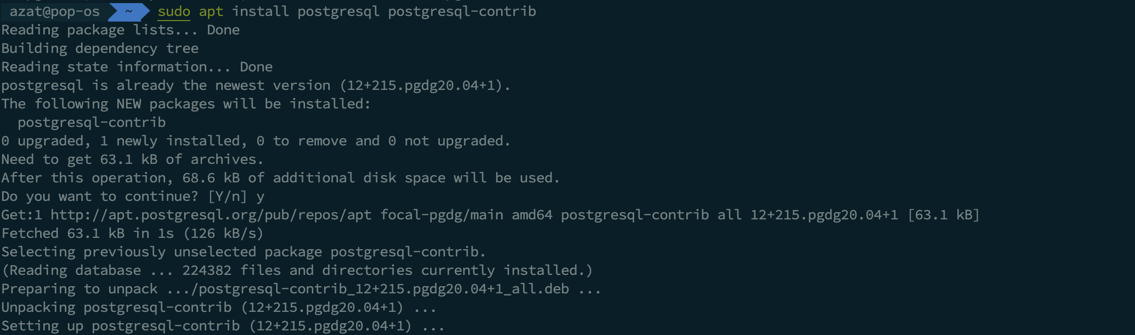
sudo apt install postgresql postgresql-contrib

Step 2: Using PostgreSQL Roles and Databases

The installation procedure created a user account called postgres that is associated with the default Postgres role. In order to use Postgres, you can log into that account.

There are a few ways to utilize this account to access Postgres.

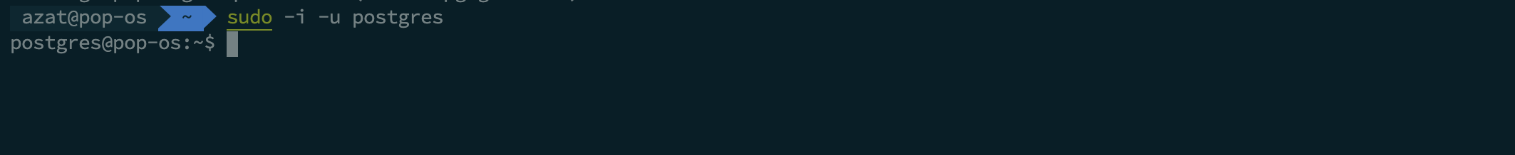
Switching Over to the Postgres Account

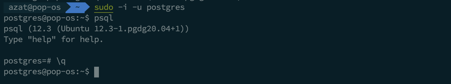
Switch over to the postgres account on your server by typing:

sudo -i -u postgres

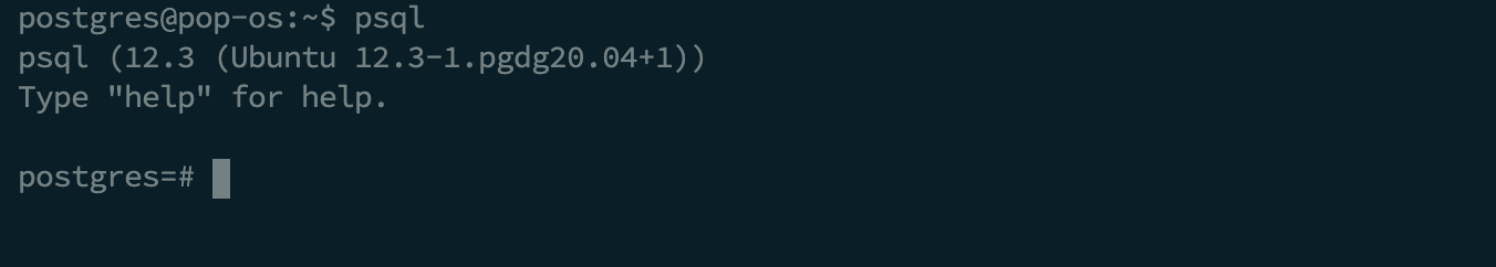
You can now access the PostgreSQL prompt immediately by typing:

psql

Exit out of the PostgreSQL prompt by typing:

\q

Step 3: Creating a New Role

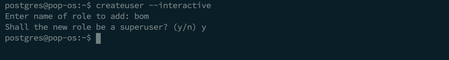
Currently, you just have the postgres role configured within the database. You can create new roles from the command line with the createrole command. The --interactive flag will prompt you for the name of the new role and also ask whether it should have superuser permissions.

If you are logged in as the postgres account, you can create a new user by typing:

createuser --interactive

If, instead, you prefer to use sudo for each command without switching from your normal account, type:

sudo -u postgres createuser --interactive

Step 4: Create a New Database

Another assumption that the Postgres authentication system makes by default is that for any role used to log in, that role will have a database with the same name which it can access.

means that , a role is somehow can be used as a saperate name for the project. for example the bom user (role) is a user which has a bom for the bom project

This means that if the user you created in the last section is called sammy, that role will attempt to connect to a database which is also called “sammy” by default. You can create the appropriate database with the createdb command.

If you are logged in as the postgres account, you would type something like:

createdb mydb

If, instead, you prefer to use sudo for each command without switching from your normal account, you would type:

sudo -u postgres createdb mydb

This flexibility provides multiple paths for creating databases as needed.

Step 5: Opening a Postgres Prompt with the New Role

To log in with ident based authentication, you’ll need a Linux user with the same name as your Postgres role and database.

If you don’t have a matching Linux user available, you can create one with the adduser command. You will have to do this from your non-root account with sudo privileges (meaning, not logged in as the postgres user):

sudo adduser sammy

Once this new account is available, you can either switch over and connect to the database by typing:

sudo -i -u sammy
psql

Or, you can do this inline:

sudo -u sammy psql

This command will log you in automatically, assuming that all of the components have been properly configured.

If you want your user to connect to a different database, you can do so by specifying the database like this:

psql -d postgres

Once logged in, you can get check your current connection information by typing:

\conninfo

Windows

PostgreSQL Terms

Architecture

In database jargon, PostgreSQL uses a client/server model. A PostgreSQL session consists of the following cooperating processes (programs):

• Server - A server process, which manages the database files, accepts connections to the database from client applications, and performs database actions on behalf of the clients. The database server program is called postgres.
• Client - The user’s client (frontend) application that wants to perform database operations. Client applications can be very diverse in nature: a client could be a text-oriented tool, a graphical application, a web server that accesses the database to display web pages, or a specialized database maintenance tool. Some client applications are supplied with the PostgreSQL distribution; most are developed by users.

1. The client and the server can be on different hosts.
2. In the obove case they communicate over a TCP/IP network.

The PostgreSQL server can handle multiple concurrent connections from clients. To achieve this it starts (“forks”) a new process for each connection. From that point on, the client and the new server process communicate without intervention by the original postgres process. Thus, the master server process is always running, waiting for client connections, whereas client and associated server processes come and go. (All of this is of course invisible to the user. We only mention it here for completeness.)

1. master process of postgres always runs and waiting for clinet connection
2. the master starts (forks) a new process for each connection.

Creating a Database

(PostgreSQL user accounts are distinct from operating system user accounts.)

You will need to become the operating system user under which PostgreSQL was installed (usually postgres) to create the first user account. It could also be that you were assigned a PostgreSQL user name that is different from your operating system user name; in that case you need to use the -U switch or set the PGUSER environment variable to specify your PostgreSQL user name.

Using Default System Username as Database Name

createdb

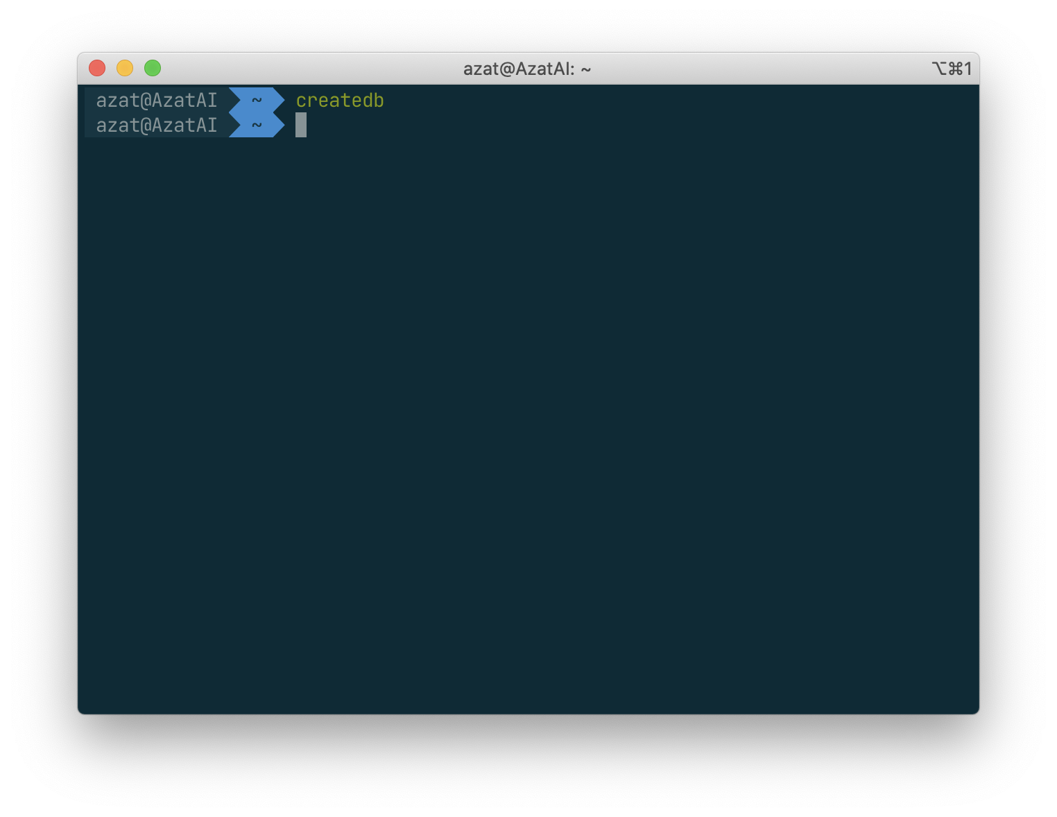
The command is just run in the terminal. Without entering any other interfaces.

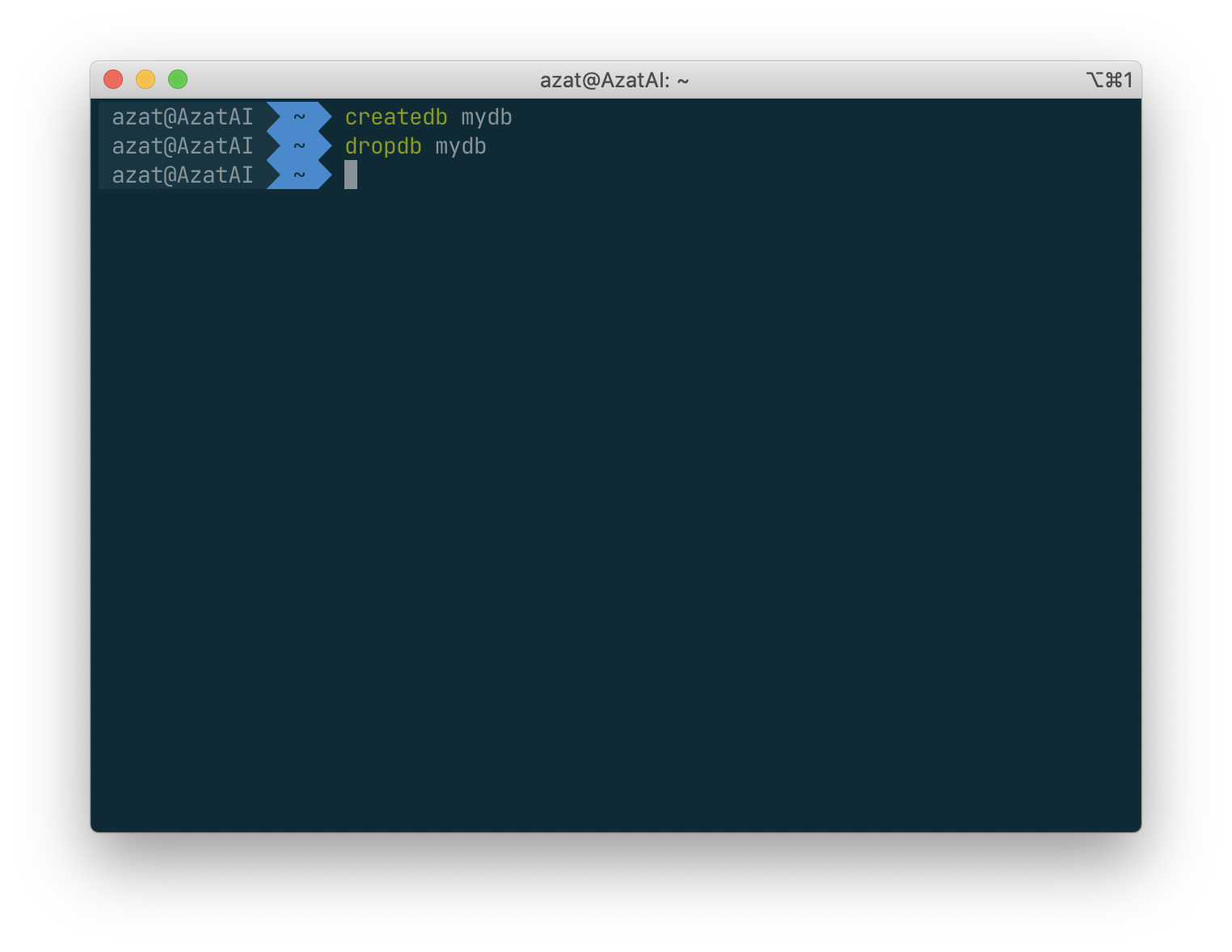
Creating Database With a Name

createdb mydb

Removing (Dropping) a Database

dropdb mydb

Accessing a Database

Once you have created a database, you can access it by:

• Running the PostgreSQL interactive terminal program, called psql, which allows you to interactively enter, edit, and execute SQL commands.
• Using an existing graphical frontend tool like pgAdmin or an office suite with ODBC or JDBC support to create and manipulate a database. These possibilities are not covered in this tutorial.
• Writing a custom application, using one of the several available language bindings. These possibilities are discussed further in Part IV.

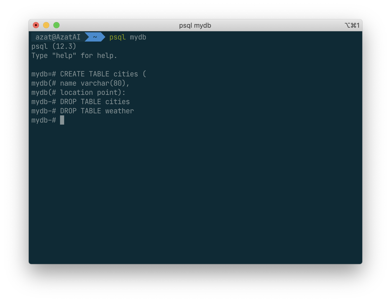
You probably want to start up psql to try the examples in this tutorial. It can be activated for the mydb database by typing the command:

psql mydb

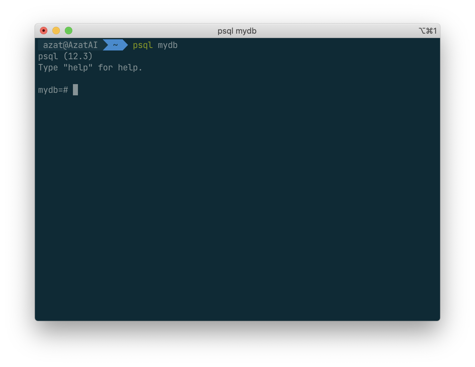
If you do not supply the database name then it will default to your user account name.

In psql, you will be greeted with the following message:

psql (12.3)
Type "help" for help.

mydb=>

Notice the => that means current user is a normal database user

The last line could also be:

mydb=#

That would mean you are a database superuser, which is most likely the case if you installed the PostgreSQL instance yourself.

Being a superuser means that you are not subject to access controls.

some other commands :

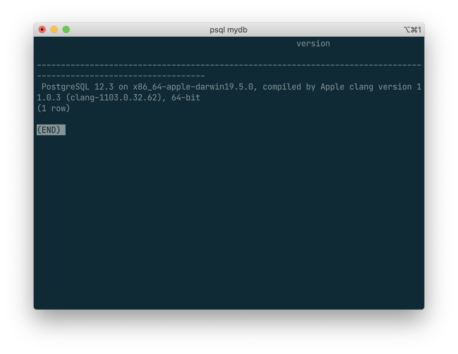
SELECT version();

Result :

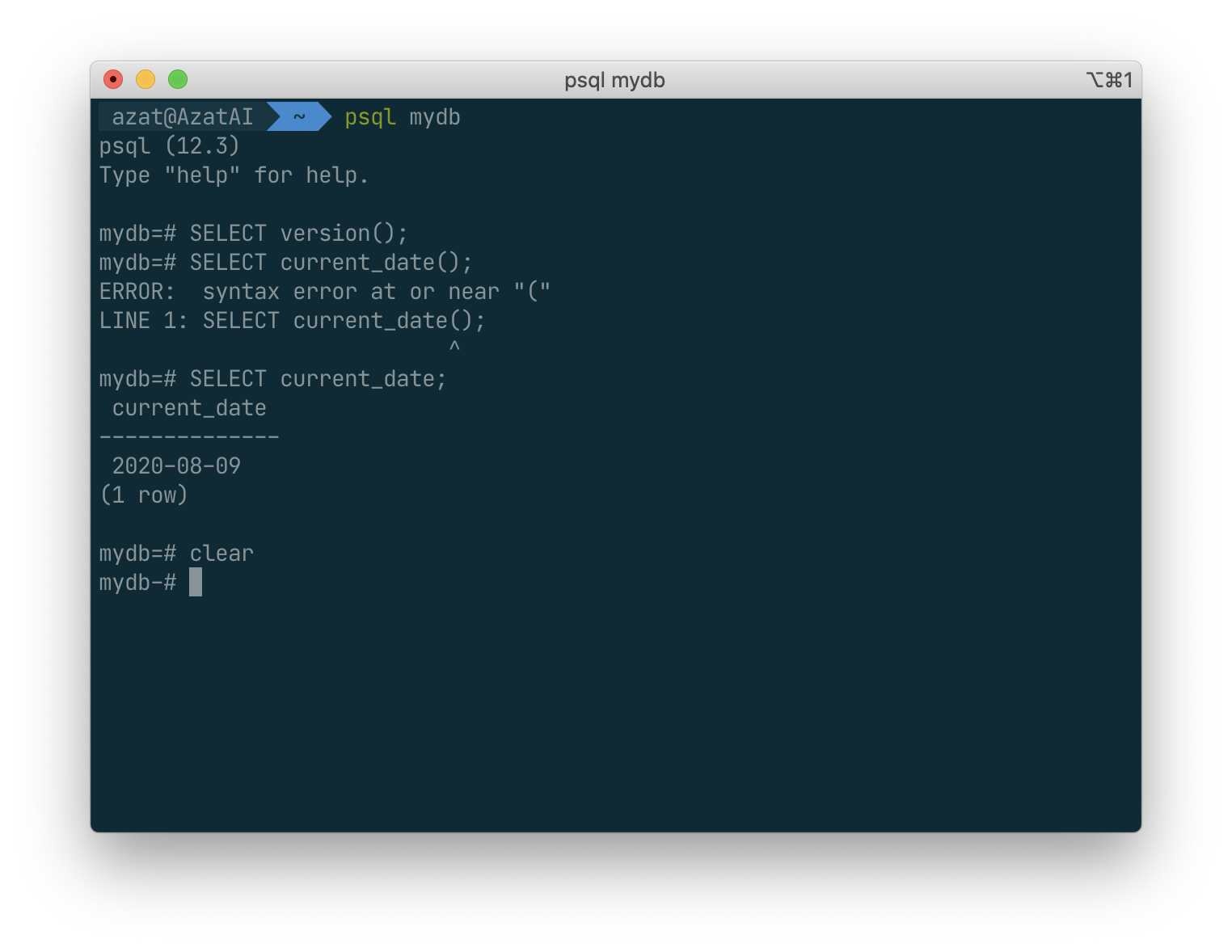
SELECT current_data();

result :

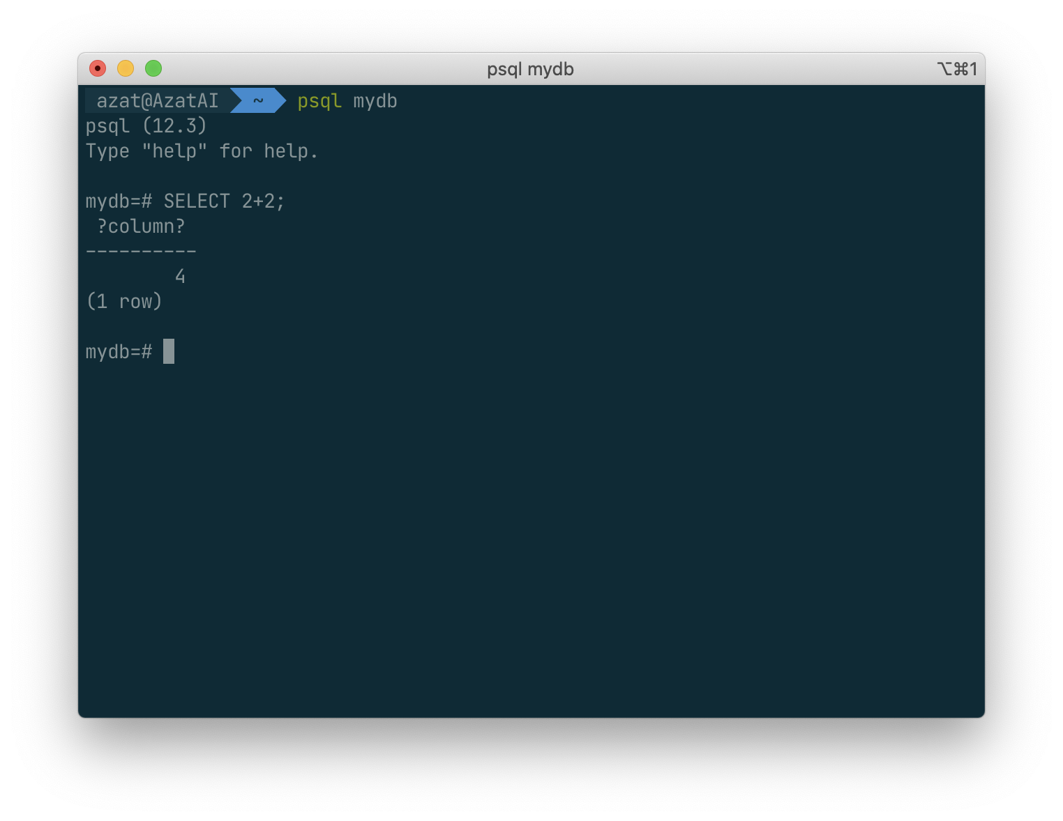
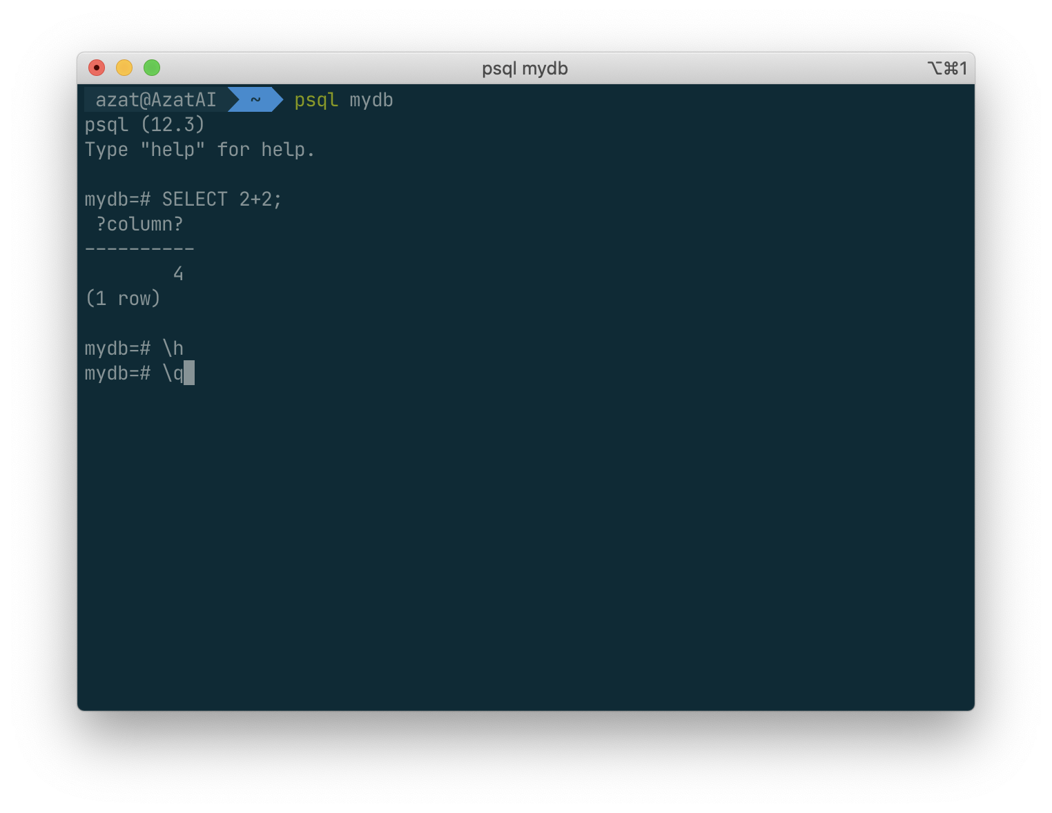
SELECT 2+2;

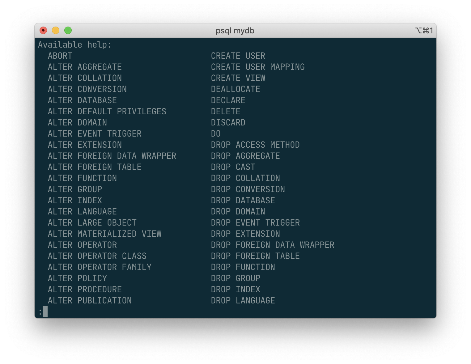
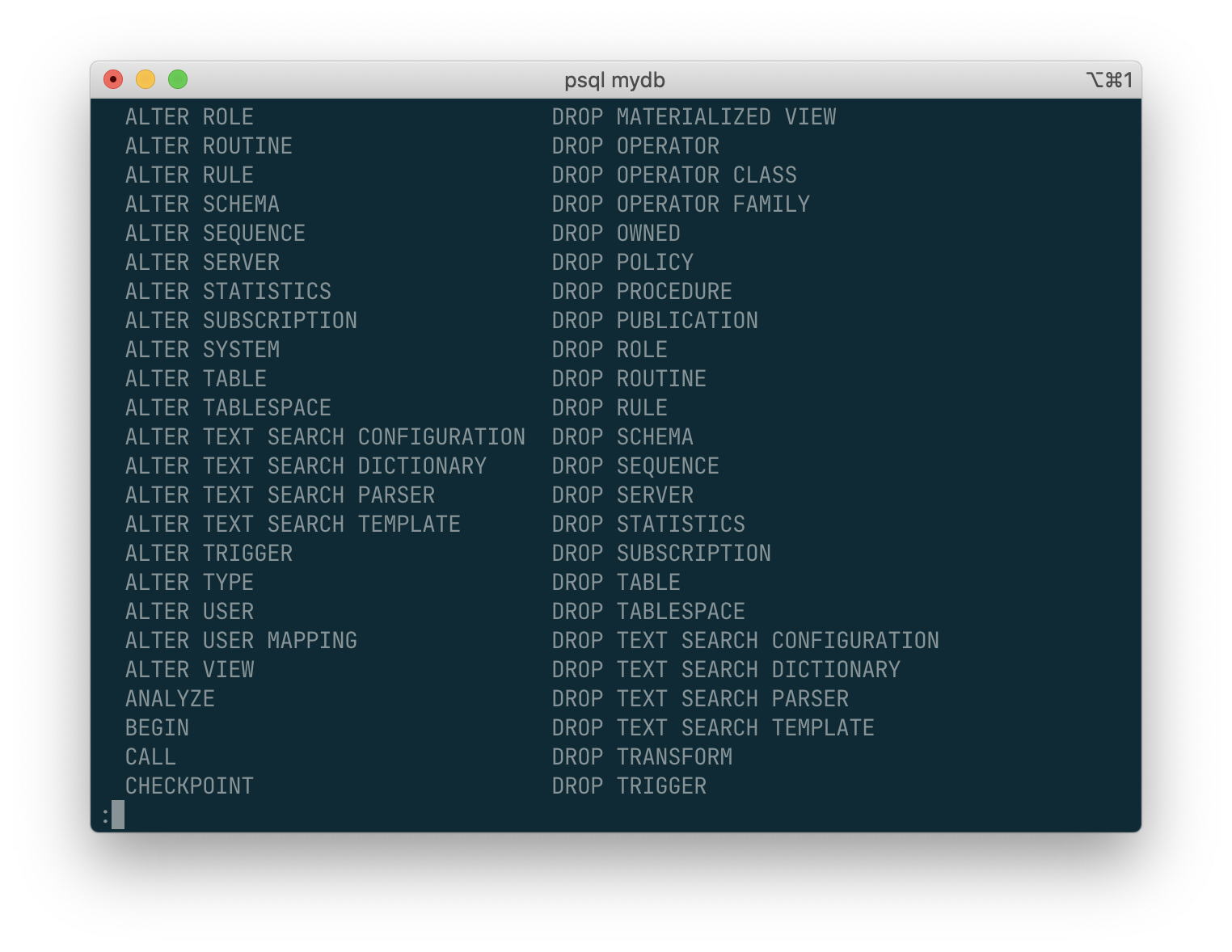
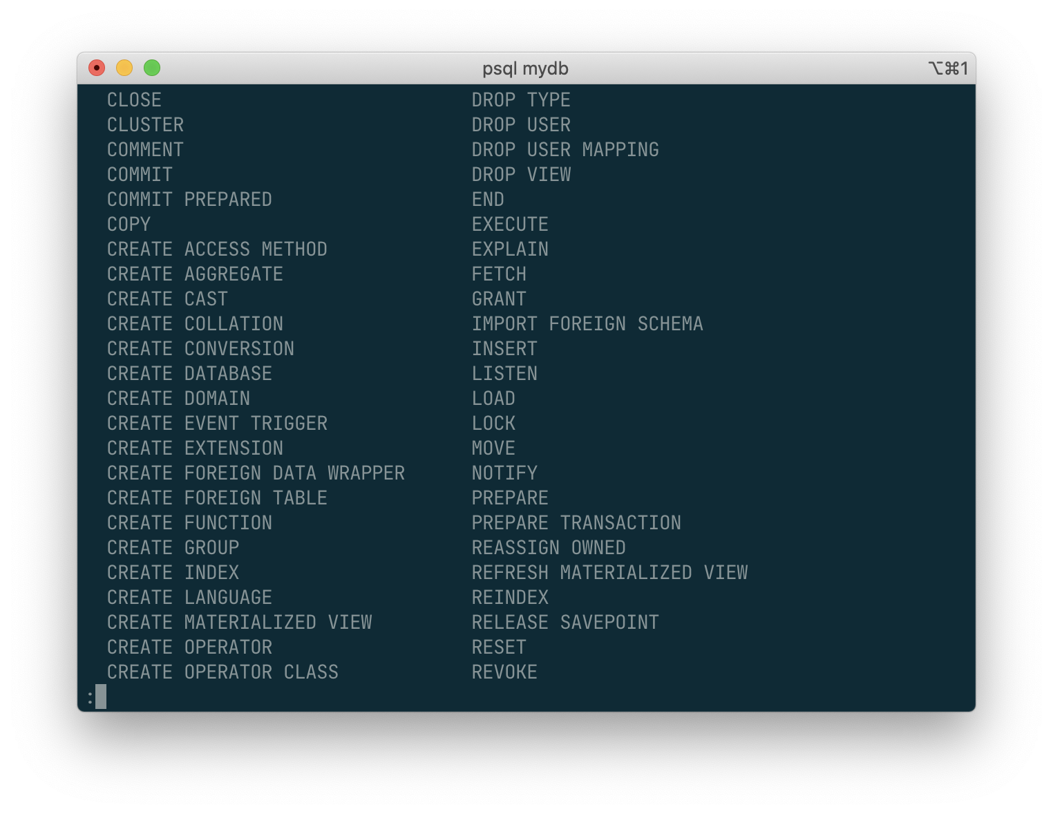
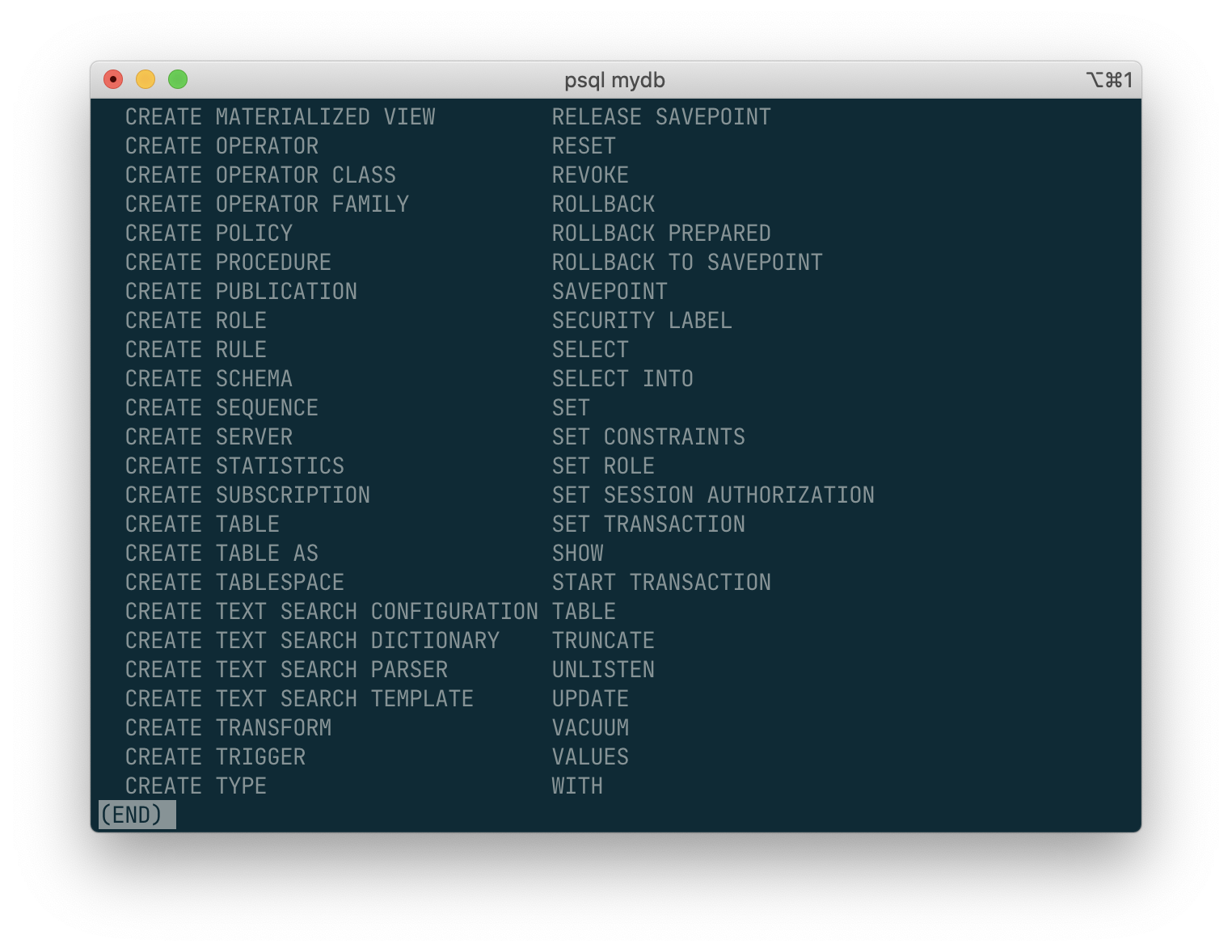
The psql program has a number of internal commands that are not SQL commands. They begin with the backslash character, “\”. For example, you can get help on the syntax of various PostgreSQL SQL commands by typing:

\h

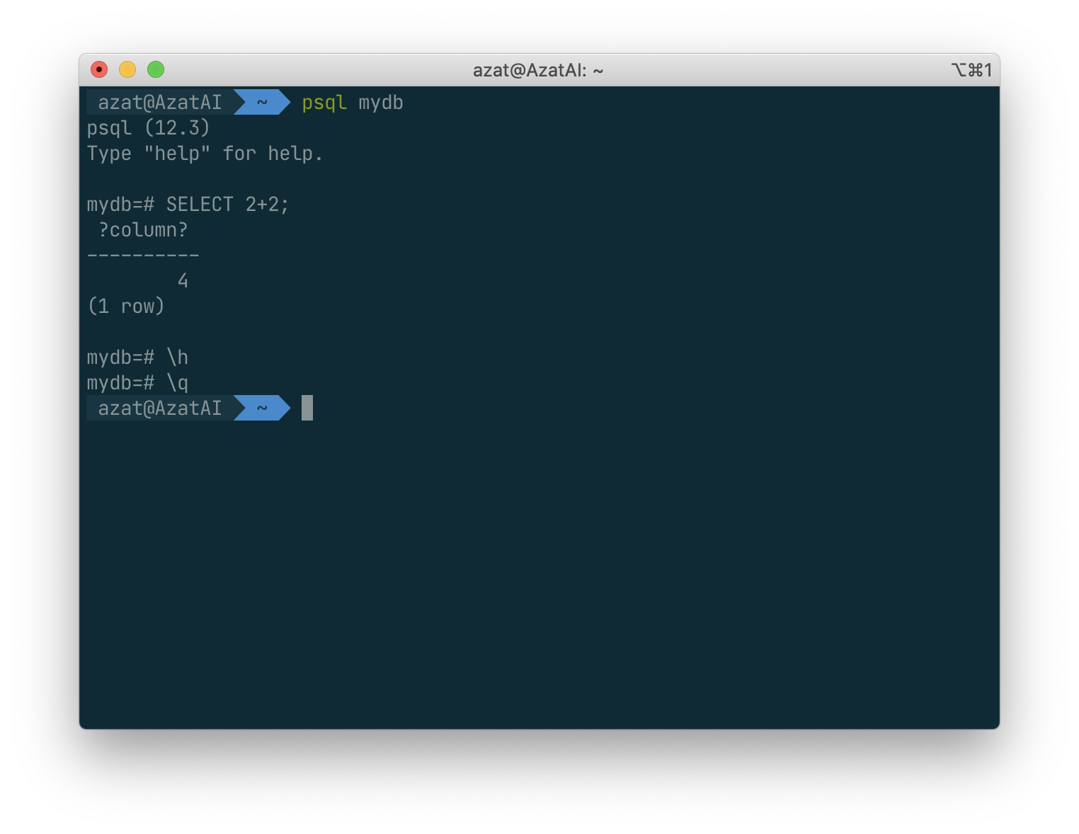
To get out of psql, type:

\q

The SQL Language

Concepts

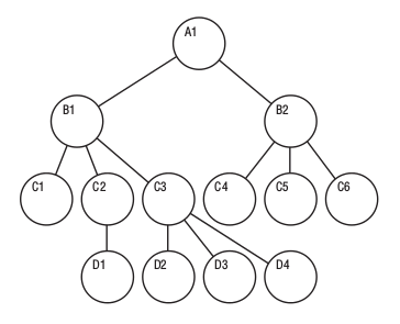
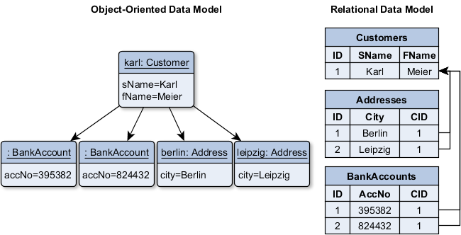
PostgreSQL is a relational database management system (RDBMS). That means it is a system for managing data stored in relations. Relation is essentially a mathematical term for table. The notion of storing data in tables is so commonplace today that it might seem inherently obvious, but there are a number of other ways of organizing databases. Files and directories on Unix-like operating systems form an example of a hierarchical database. A more modern development is the object-oriented database.

1. PostgreSQL is a relational database management system (RDBMS)
2. Relation is essentially a mathematical term for table
3. Files and directories on Unix-like operating system form an example of hierachical database.

hierachical database :

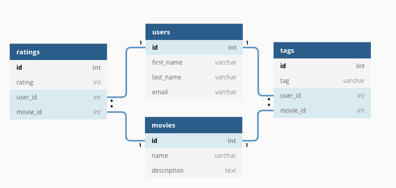
relational database:

object-oriented database:

Each table is a named collection of rows. Each row of a given table has the same set of named columns, and each column is of a specific data type. Whereas columns have a fixed order in each row, it is important to remember that SQL does not guarantee the order of the rows within the table in any way (although they can be explicitly sorted for display).

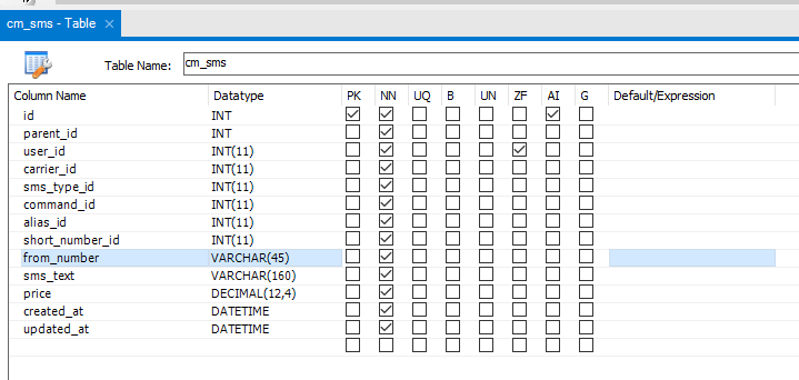
Database table:

Column datatypes:

Tables are grouped into databases, and a collection of databases managed by a single PostgreSQL server instance constitutes a database cluster.

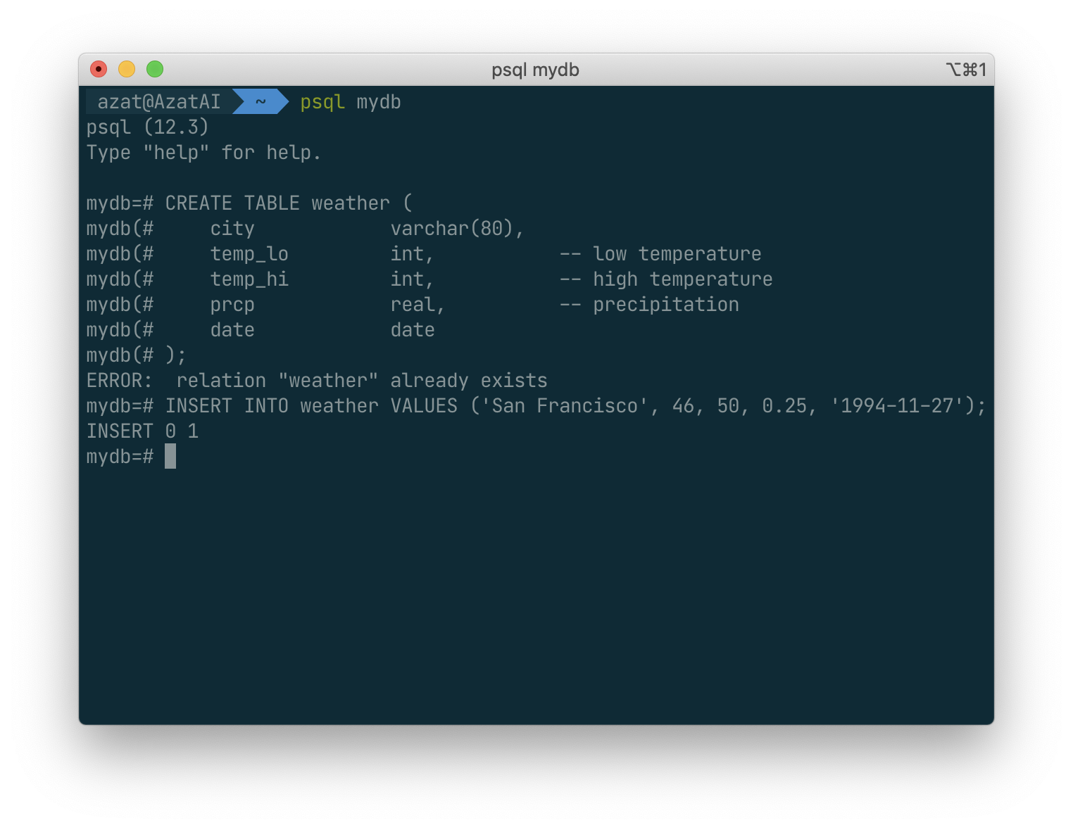
Creating a New Table

Tis is all are actions inside a specific database, here it is mydb

You can create a new table by specifying the table name, along with all column names and their types:

The point type is an example of a PostgreSQL-specific data type.

Finally, it should be mentioned that if you don’t need a table any longer or want to recreate it differently you can remove it using the following command:

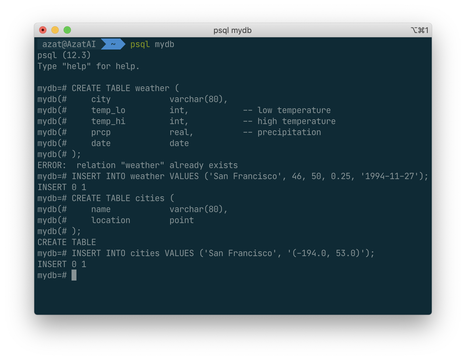
Populating a Table With Rows

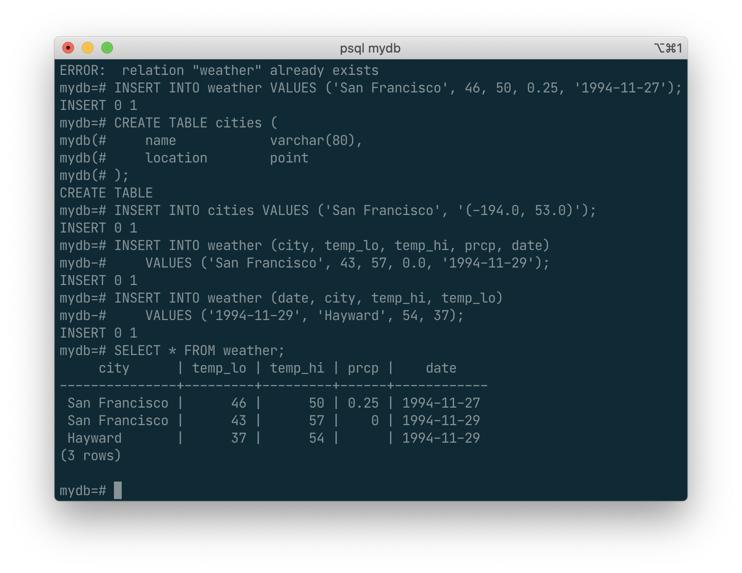
The INSERT statement is used to populate a table with rows:

Note that all data types use rather obvious input formats. Constants that are not simple numeric values usually must be surrounded by single quotes ('), as in the example.

The point type requires a coordinate pair as input, as shown here:

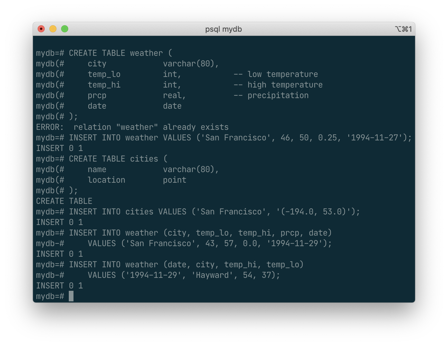
The syntax used so far requires you to remember the order of the columns. An alternative syntax allows you to list the columns explicitly:

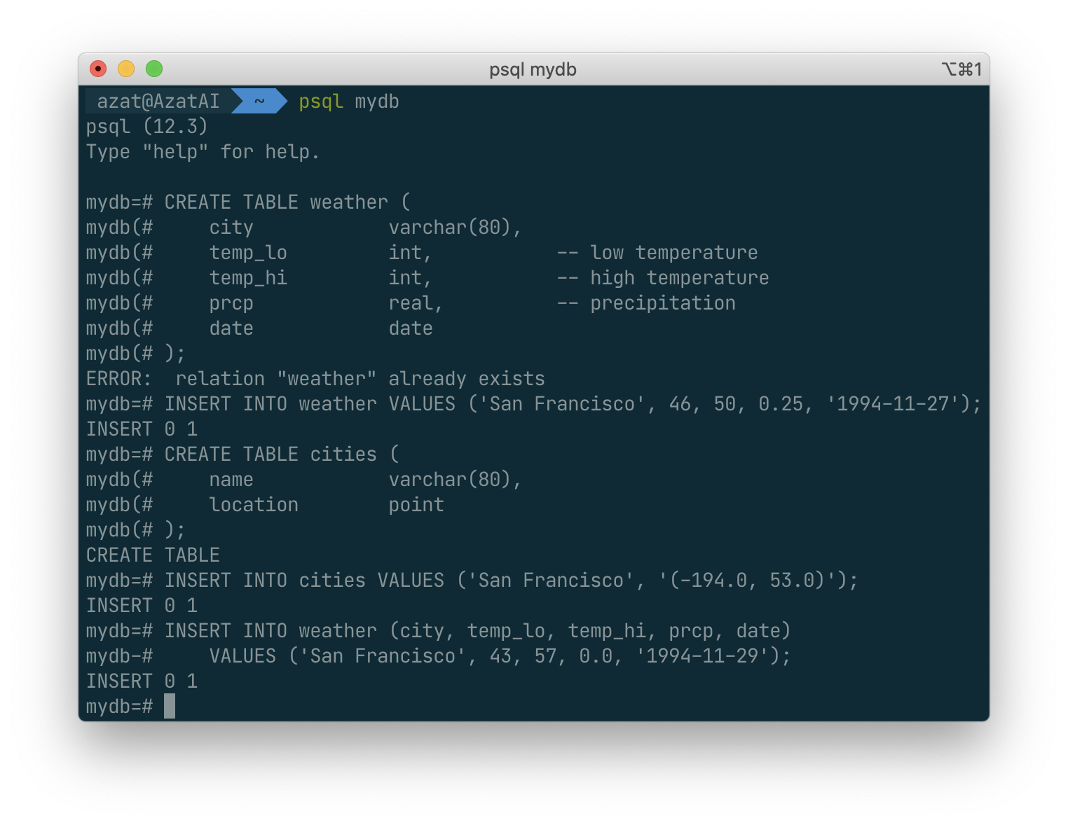
You can list the columns in a different order if you wish or even omit some columns, e.g., if the precipitation is unknown:

You could also have used COPY to load large amounts of data from flat-text files. This is usually faster because the COPY command is optimized for this application while allowing less flexibility than INSERT. An example would be:

COPY weather FROM '/home/user/weather.txt';

where the file name for the source file must be available on the machine running the backend process, not the client, since the backend process reads the file directly. You can read more about the COPY command in COPY.

Querying a Table

To retrieve data from a table, the table is queried. An SQL SELECT statement is used to do this. The statement is divided into a select list (the part that lists the columns to be returned), a table list (the part that lists the tables from which to retrieve the data), and an optional qualification (the part that specifies any restrictions). For example, to retrieve all the rows of table weather, type:

SELECT statement :

• select list (the coulumns to be returned)
• table list (table from which to retrieve data)
• qualification (specifies any restrictions)

SELECT * FROM weather;

Here * is a shorthand for “all columns”. [2] So the same result would be had with:

SELECT city, temp_lo, temp_hi, prcp, date FROM weather;

You can write expressions, not just simple column references, in the select list. For example, you can do:

SELECT city, (temp_hi+temp_lo)/2 AS temp_avg, date FROM weather;

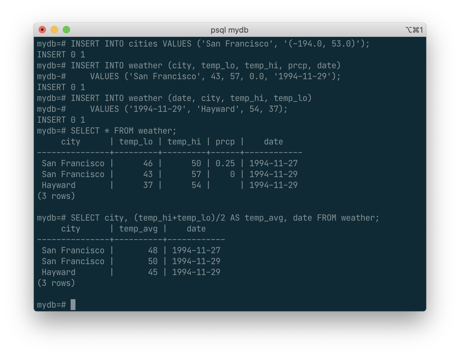
Notice how the AS clause is used to relabel the output column. (The AS clause is optional.)

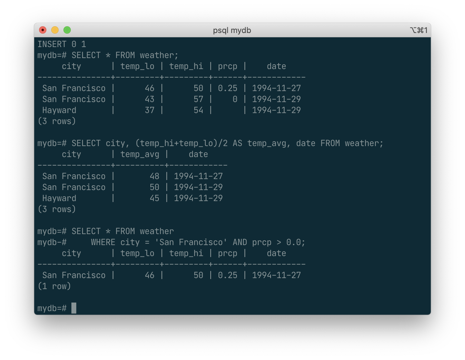
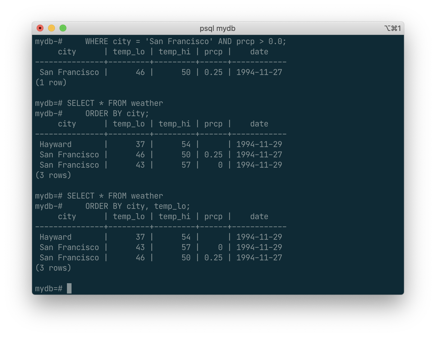
A query can be “qualified” by adding a WHERE clause that specifies which rows are wanted. The WHERE clause contains a Boolean (truth value) expression, and only rows for which the Boolean expression is true are returned. The usual Boolean operators (AND, OR, and NOT) are allowed in the qualification. For example, the following retrieves the weather of San Francisco on rainy days:

SELECT * FROM weather
    WHERE city = 'San Francisco' AND prcp > 0.0;

You can request that the results of a query be returned in sorted order:

SELECT * FROM weather
    ORDER BY city;

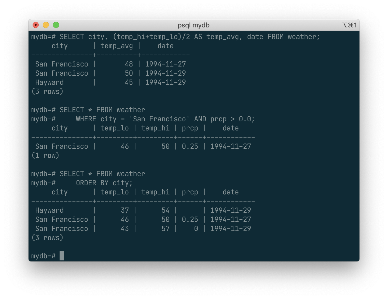
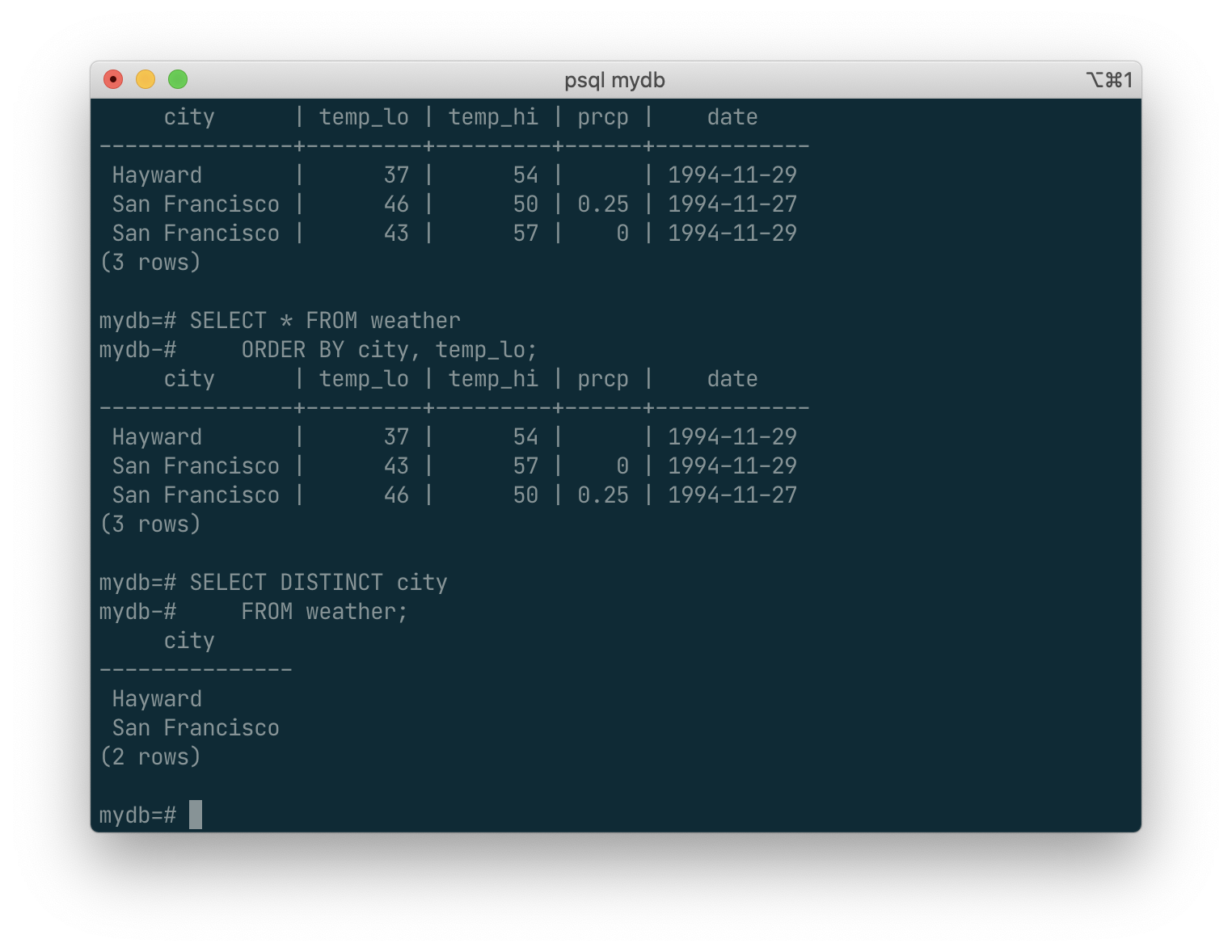
In this example, the sort order isn’t fully specified, and so you might get the San Francisco rows in either order. But you’d always get the results shown above if you do:

SELECT * FROM weather
    ORDER BY city, temp_lo;

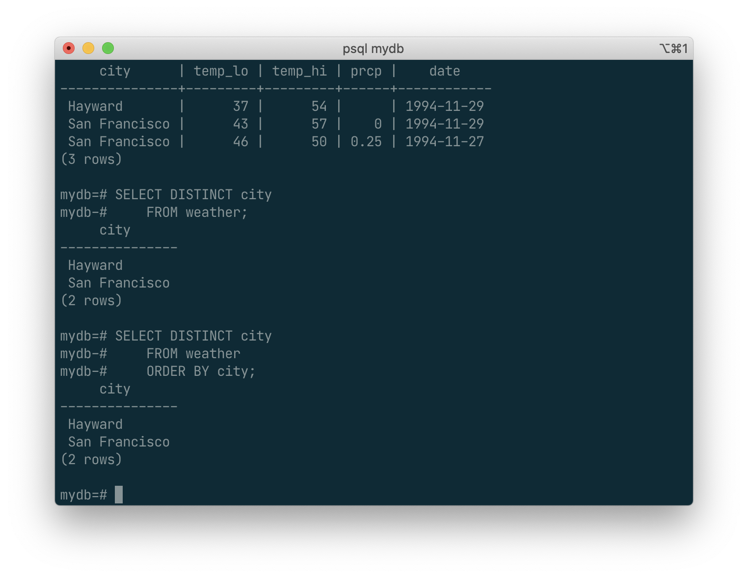
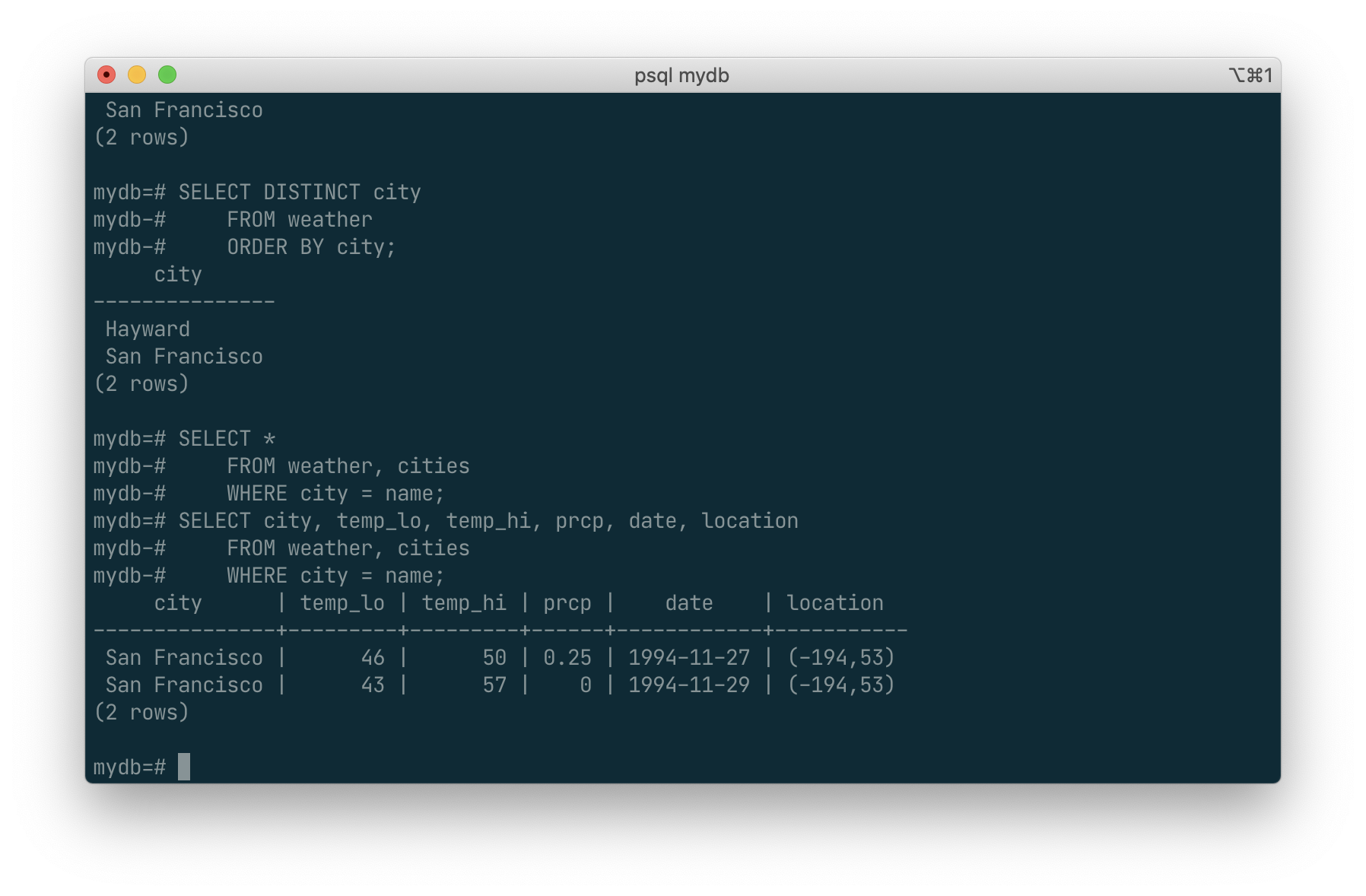
You can request that duplicate rows be removed from the result of a query:

SELECT DISTINCT city
    FROM weather;

Here again, the result row ordering might vary. You can ensure consistent results by using DISTINCT and ORDER BY together: [3]

SELECT DISTINCT city
    FROM weather
    ORDER BY city;

While SELECT * is useful for off-the-cuff queries, it is widely considered bad style in production code, since adding a column to the table would change the results.

Join Between Tables

Thus far, our queries have only accessed one table at a time. Queries can access multiple tables at once, or access the same table in such a way that multiple rows of the table are being processed at the same time. A query that accesses multiple rows of the same or different tables at one time is called a join query. As an example, say you wish to list all the weather records together with the location of the associated city. To do that, we need to compare the city column of each row of the weather table with the name column of all rows in the cities table, and select the pairs of rows where these values match.

This would be accomplished by the following query:

SELECT *
    FROM weather, cities
    WHERE city = name;

Observe two things about the result set:

• There is no result row for the city of Hayward. This is because there is no matching entry in the cities table for Hayward, so the join ignores the unmatched rows in the weather table. We will see shortly how this can be fixed.
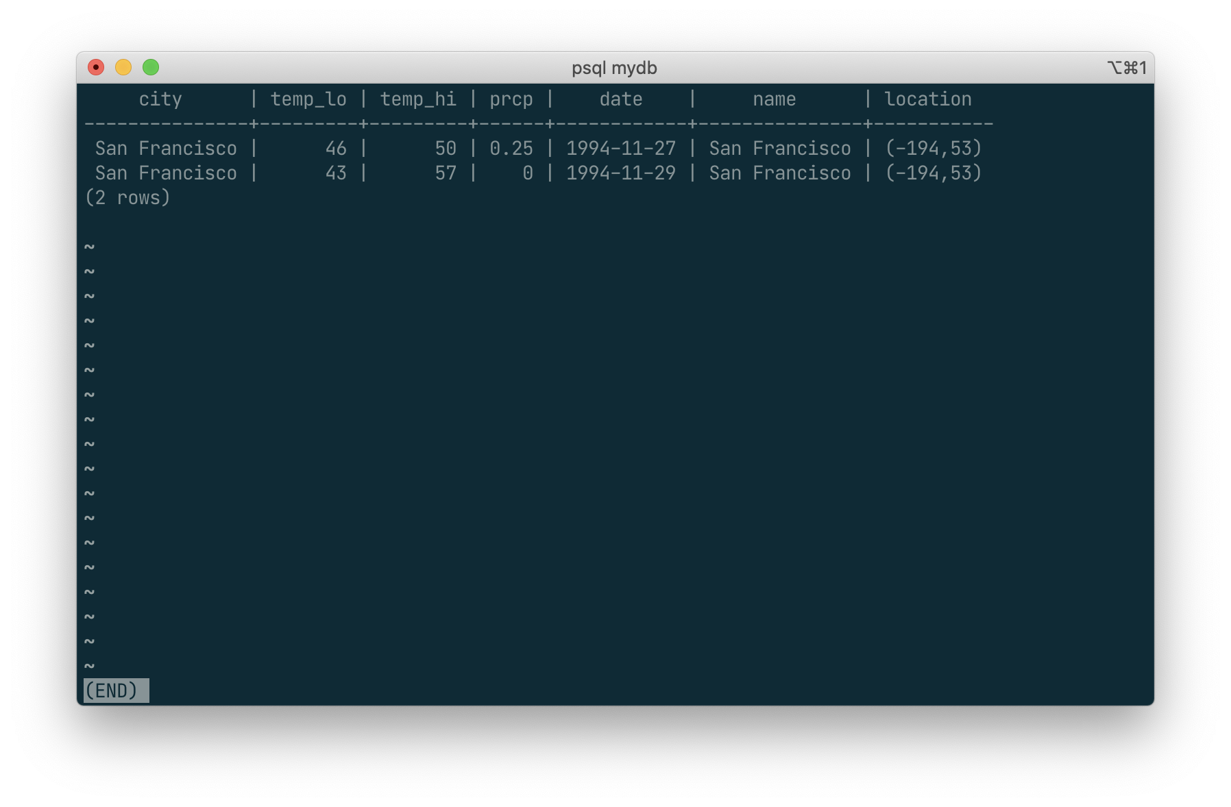
• There are two columns containing the city name. This is correct because the lists of columns from the weather and cities tables are concatenated. In practice this is undesirable, though, so you will probably want to list the output columns explicitly rather than using *:

SELECT city, temp_lo, temp_hi, prcp, date, location
    FROM weather, cities
    WHERE city = name;

Exercise: Attempt to determine the semantics of this query when the WHERE clause is omitted.

Since the columns all had different names, the parser automatically found which table they belong to. If there were duplicate column names in the two tables you’d need to qualify the column names to show which one you meant, as in:

SELECT weather.city, weather.temp_lo, weather.temp_hi,
       weather.prcp, weather.date, cities.location
    FROM weather, cities
    WHERE cities.name = weather.city;

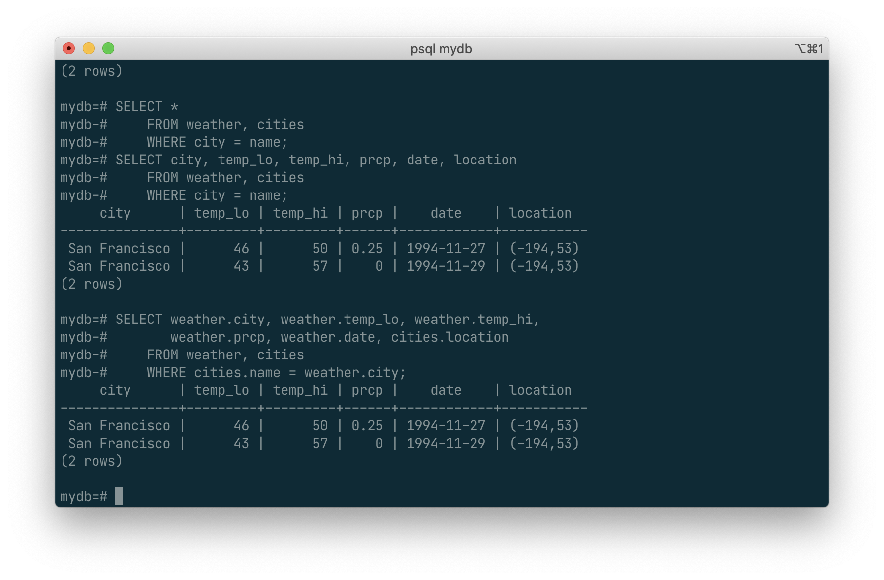
It is widely considered good style to qualify all column names in a join query, so that the query won’t fail if a duplicate column name is later added to one of the tables.

Join queries of the kind seen thus far can also be written in this alternative form:

SELECT *
    FROM weather INNER JOIN cities ON (weather.city = cities.name);

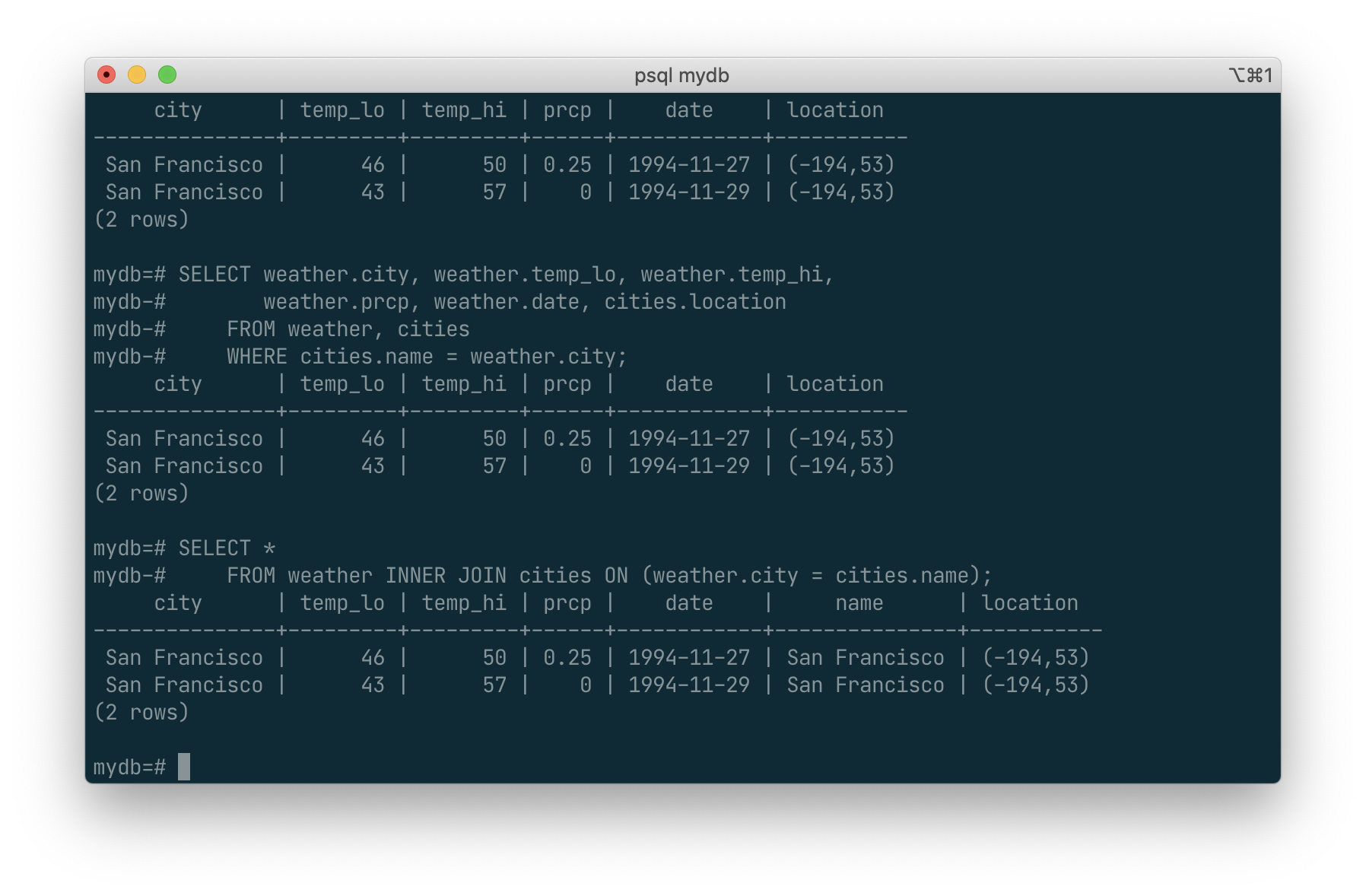
This syntax is not as commonly used as the one above, but we show it here to help you understand the following topics.

Now we will figure out how we can get the Hayward records back in. What we want the query to do is to scan the weather table and for each row to find the matching cities row(s). If no matching row is found we want some “empty values” to be substituted for the cities table’s columns. This kind of query is called an outer join. (The joins we have seen so far are inner joins.) The command looks like this:

SELECT *
    FROM weather LEFT OUTER JOIN cities ON (weather.city = cities.name);

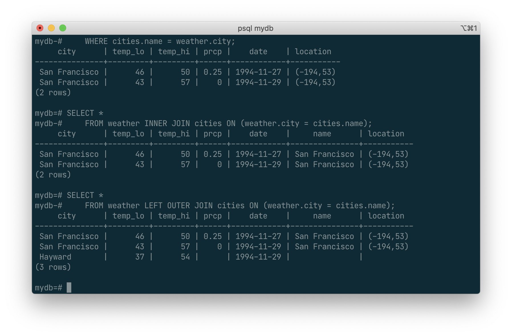
This query is called a left outer join because the table mentioned on the left of the join operator will have each of its rows in the output at least once, whereas the table on the right will only have those rows output that match some row of the left table. When outputting a left-table row for which there is no right-table match, empty (null) values are substituted for the right-table columns.

Exercise: There are also right outer joins and full outer joins. Try to find out what those do.

SELECT *
    FROM weather RIGHT OUTER JOIN cities ON (weather.city = cities.name);

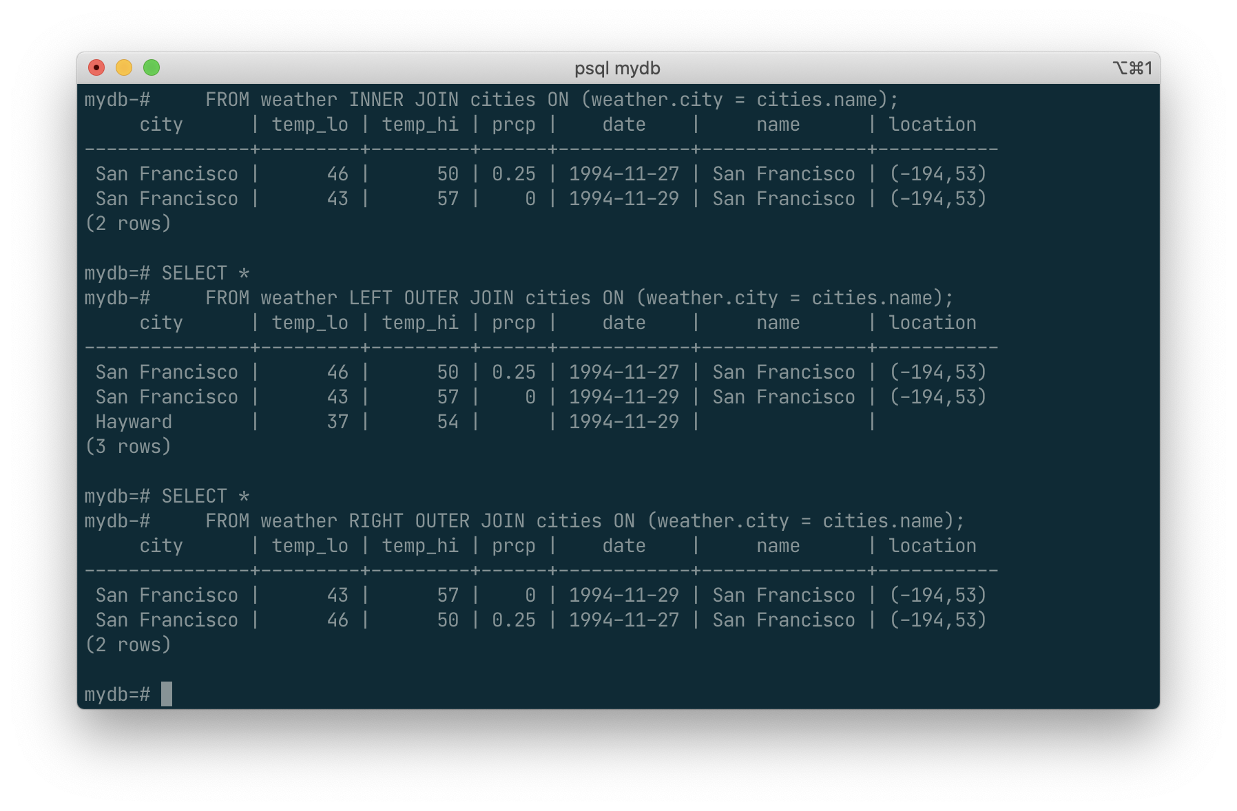
The left and right is difference the order for scan. Left scans the first table and for each of the records finds a match from the second table, while the right dose the opposite.

We can also join a table against itself. This is called a self join. As an example, suppose we wish to find all the weather records that are in the temperature range of other weather records. So we need to compare the temp_lo and temp_hi columns of each weather row to the temp_lo and temp_hi columns of all other weather rows. We can do this with the following query:

SELECT W1.city, W1.temp_lo AS low, W1.temp_hi AS high,
    W2.city, W2.temp_lo AS low, W2.temp_hi AS high
    FROM weather W1, weather W2
    WHERE W1.temp_lo < W2.temp_lo
    AND W1.temp_hi > W2.temp_hi;

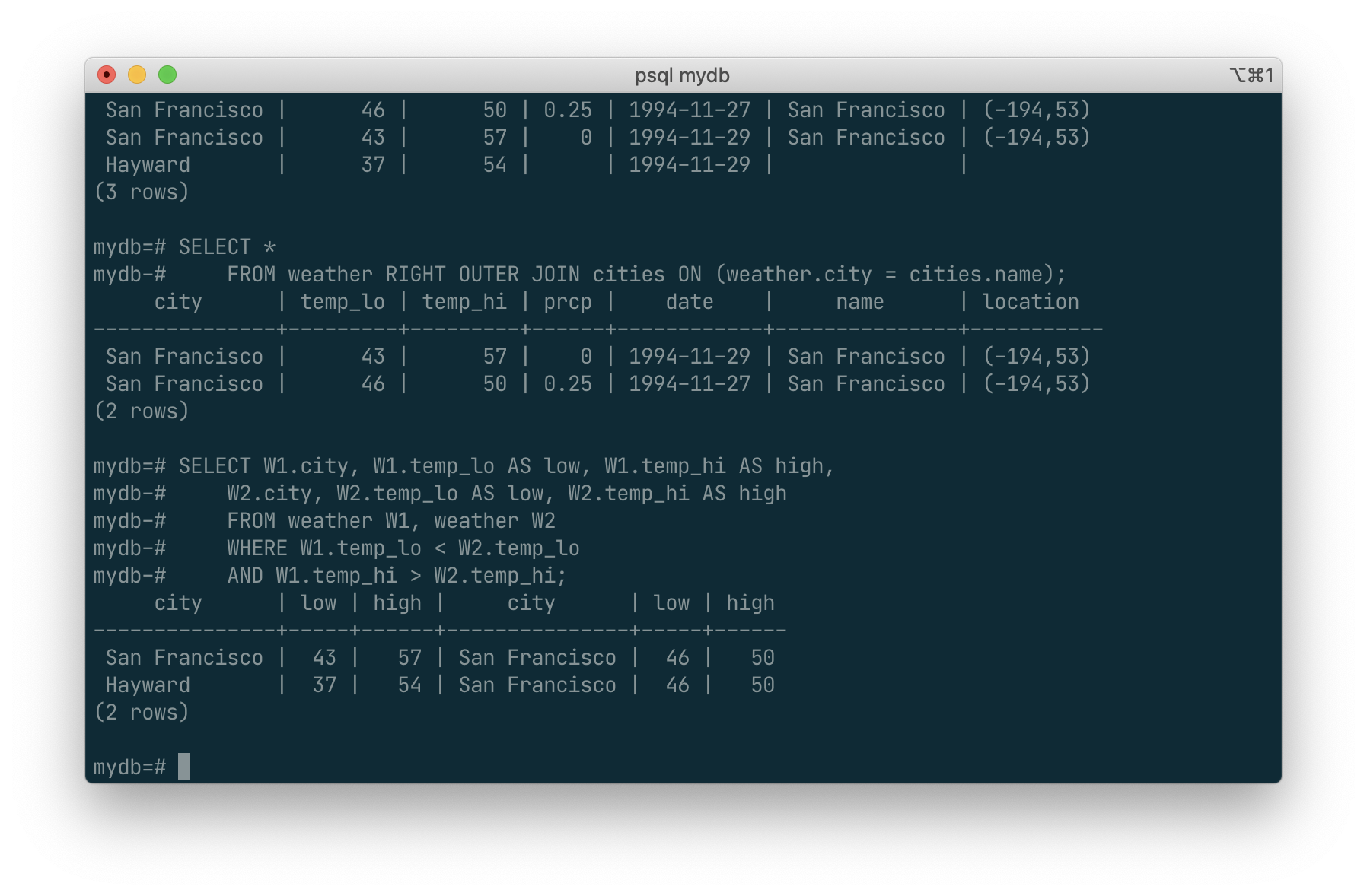
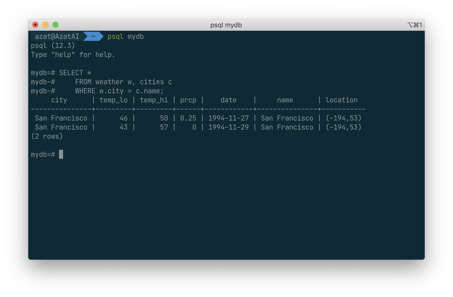
Here we have relabeled the weather table as W1 and W2 to be able to distinguish the left and right side of the join. You can also use these kinds of aliases in other queries to save some typing, e.g.:

SELECT *
    FROM weather w, cities c
    WHERE w.city = c.name;

Aggregate Function

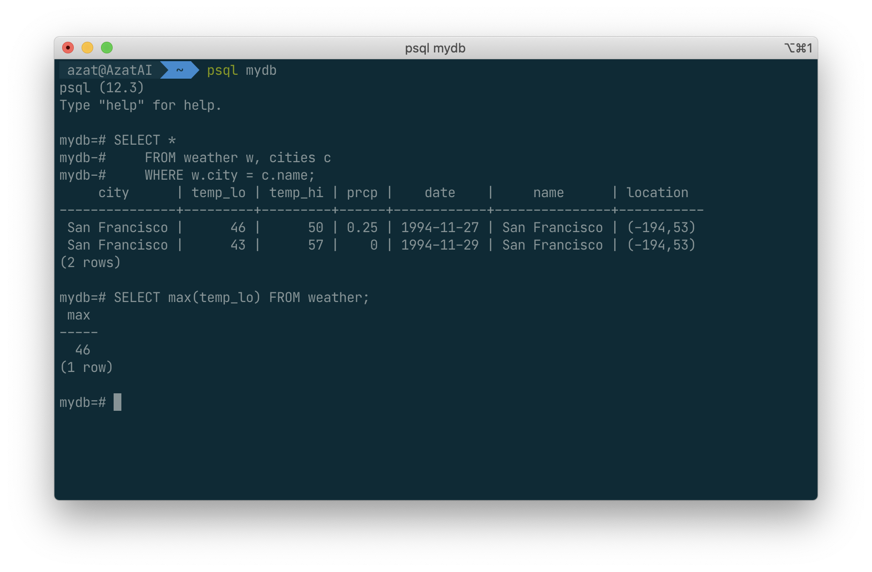
Like most other relational database products, PostgreSQL supports aggregate functions. An aggregate function computes a single result from multiple input rows. For example, there are aggregates to compute the count, sum, avg (average), max (maximum) and min (minimum) over a set of rows.

As an example, we can find the highest low-temperature reading anywhere with:

SELECT max(temp_lo) FROM weather;

If we wanted to know what city (or cities) that reading occurred in, we might try:

SELECT city FROM weather
    WHERE temp_lo = (SELECT max(temp_lo) FROM weather);

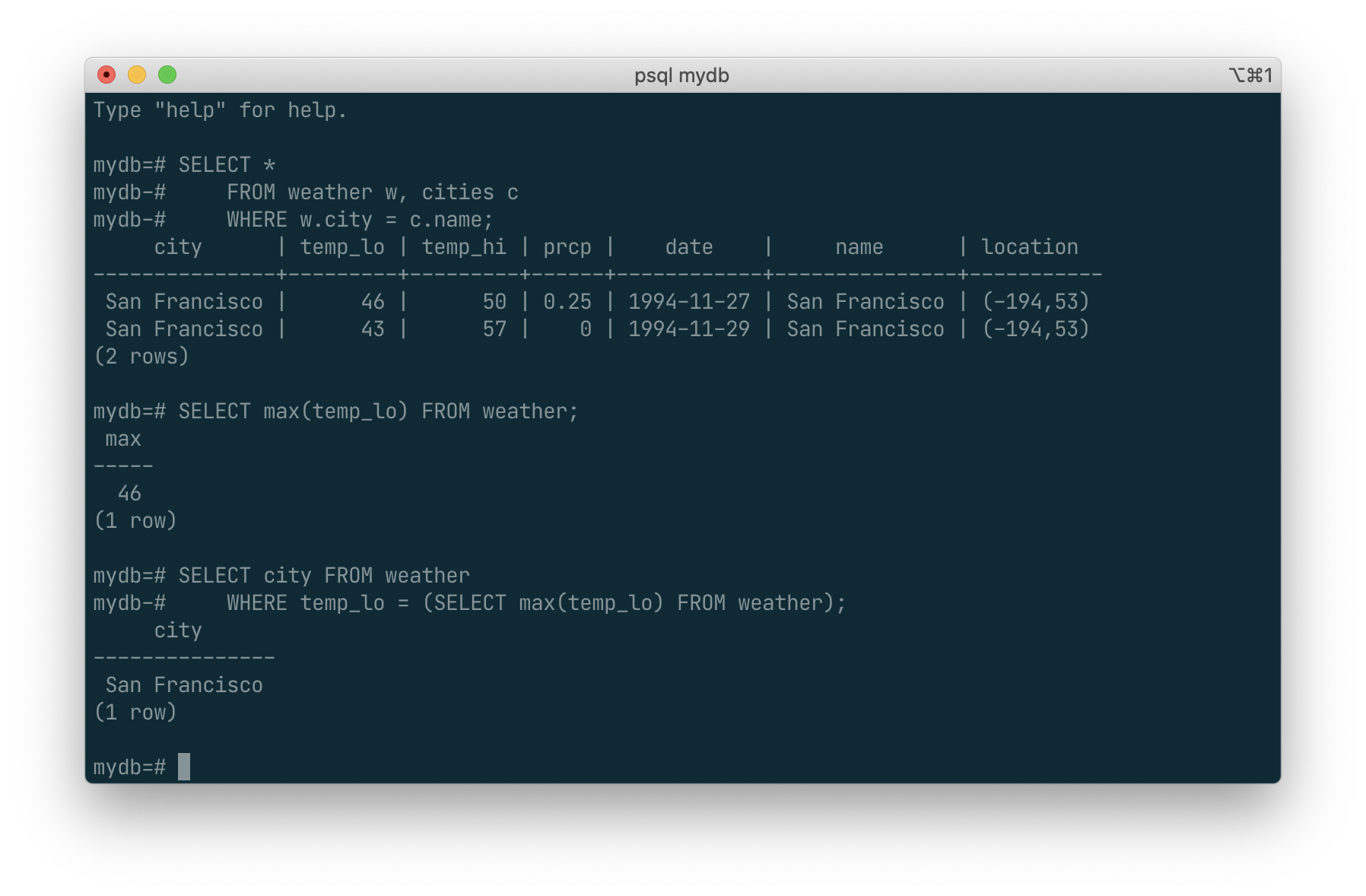
This is OK because the subquery is an independent computation that computes its own aggregate separately from what is happening in the outer query.

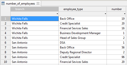
Aggregates are also very useful in combination with GROUP BY clauses. For example, we can get the maximum low temperature observed in each city with:

SELECT city, max(temp_lo)
    FROM weather
    GROUP BY city;

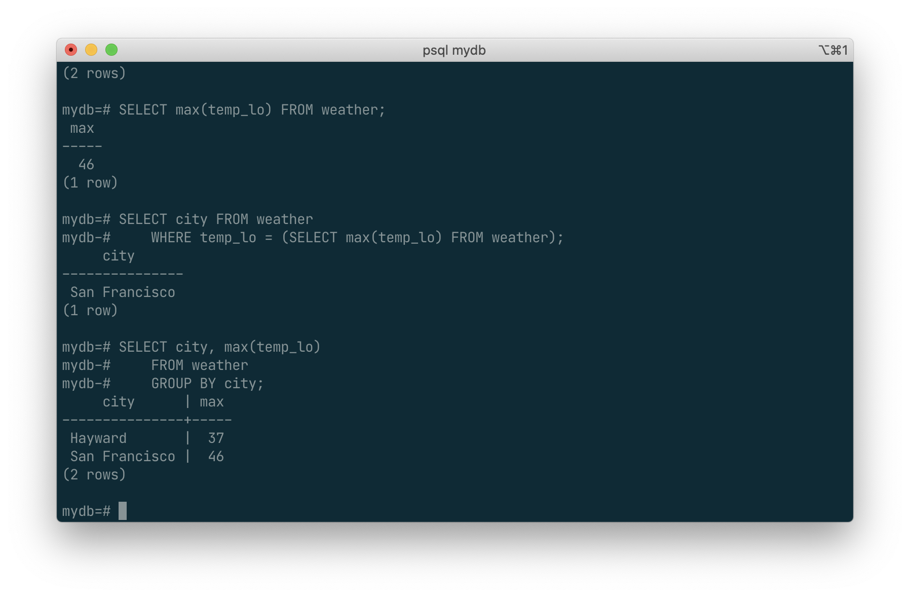
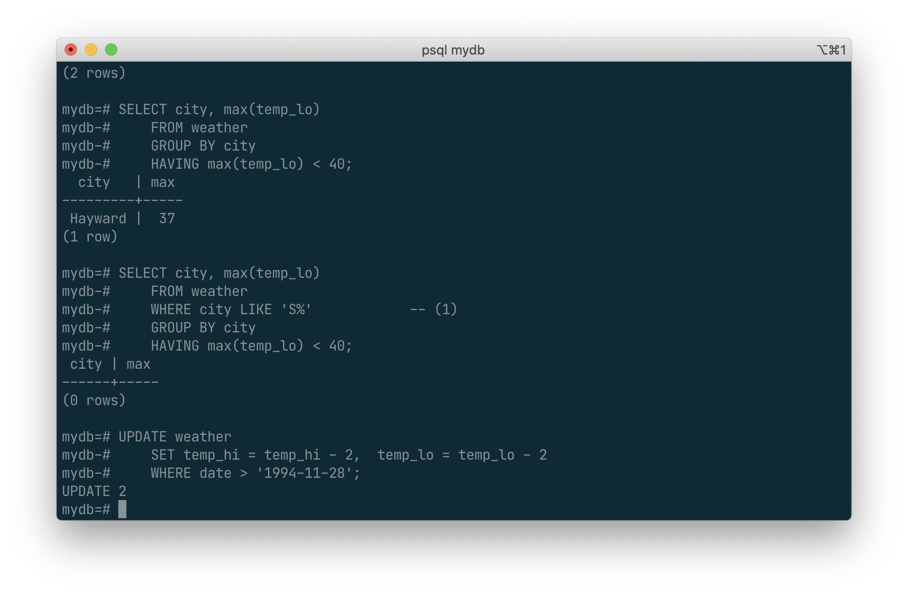
which gives us one output row per city. Each aggregate result is computed over the table rows matching that city. We can filter these grouped rows using HAVING:

SELECT city, max(temp_lo)
    FROM weather
    GROUP BY city
    HAVING max(temp_lo) < 40;

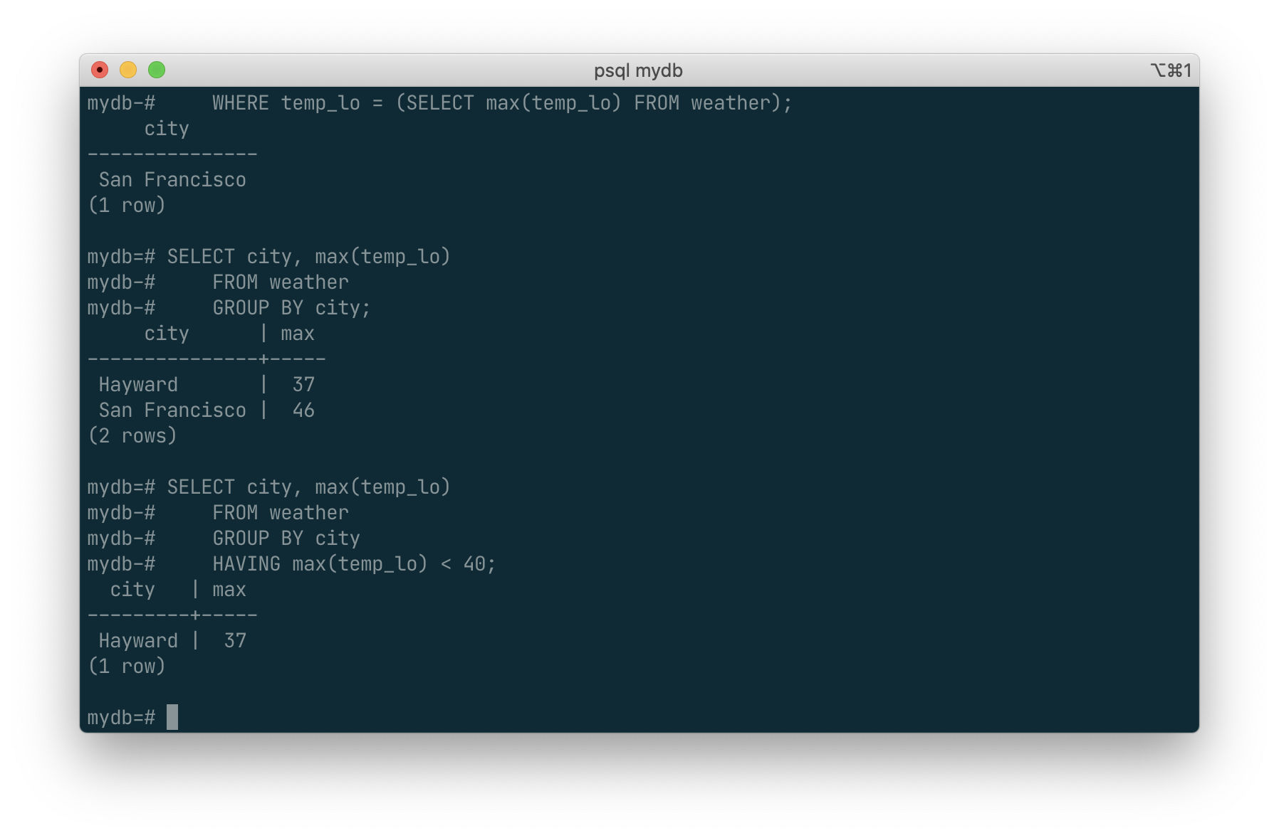
which gives us the same results for only the cities that have all temp_lo values below 40. Finally, if we only care about cities whose names begin with “S”, we might do:

SELECT city, max(temp_lo)
    FROM weather
    WHERE city LIKE 'S%'            -- (1)
    GROUP BY city
    HAVING max(temp_lo) < 40;

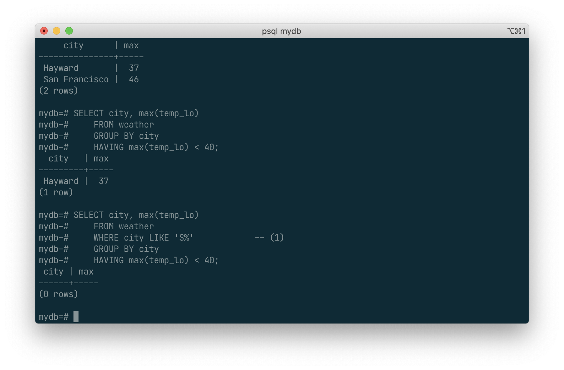
The LIKE operator does pattern matching and is explained in Section 9.7.

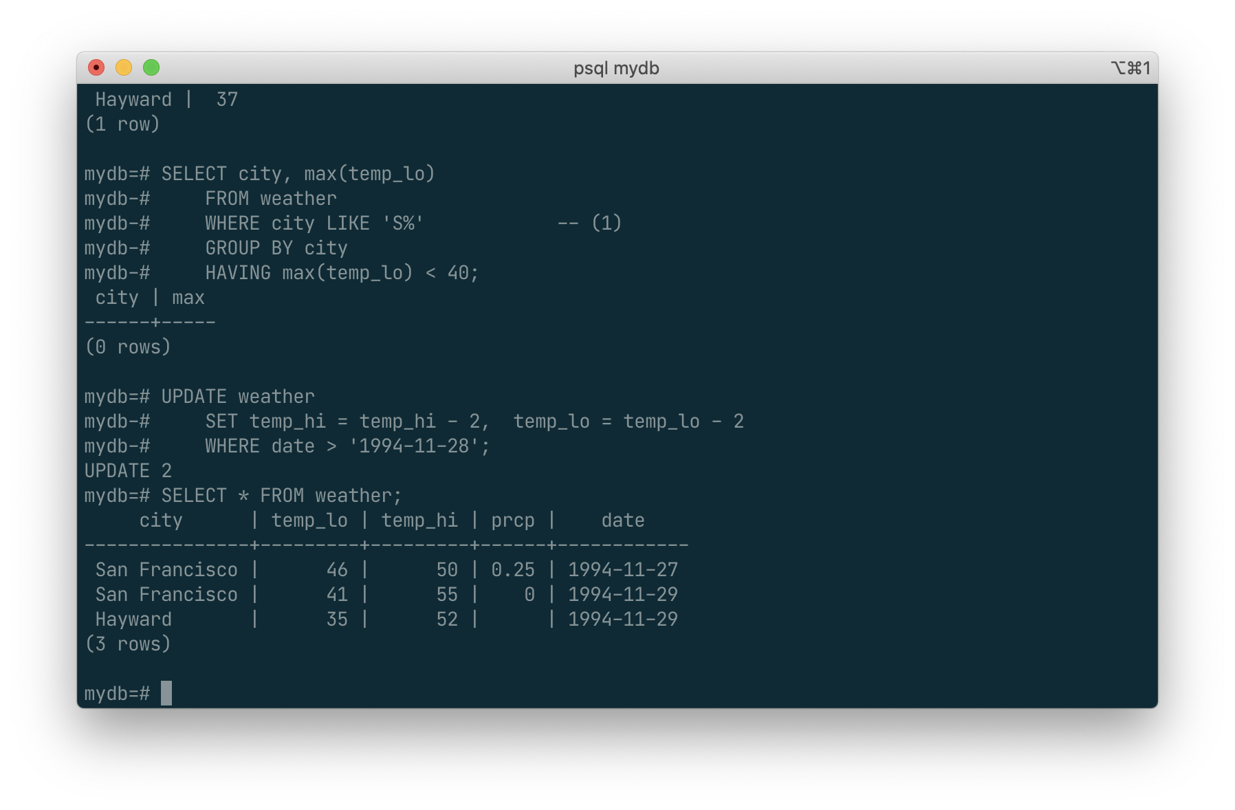
Updates

You can update existing rows using the UPDATE command. Suppose you discover the temperature readings are all off by 2 degrees after November 28. You can correct the data as follows:

UPDATE weather
    SET temp_hi = temp_hi - 2,  temp_lo = temp_lo - 2
    WHERE date > '1994-11-28';

Look at the new state of the data:

SELECT * FROM weather;

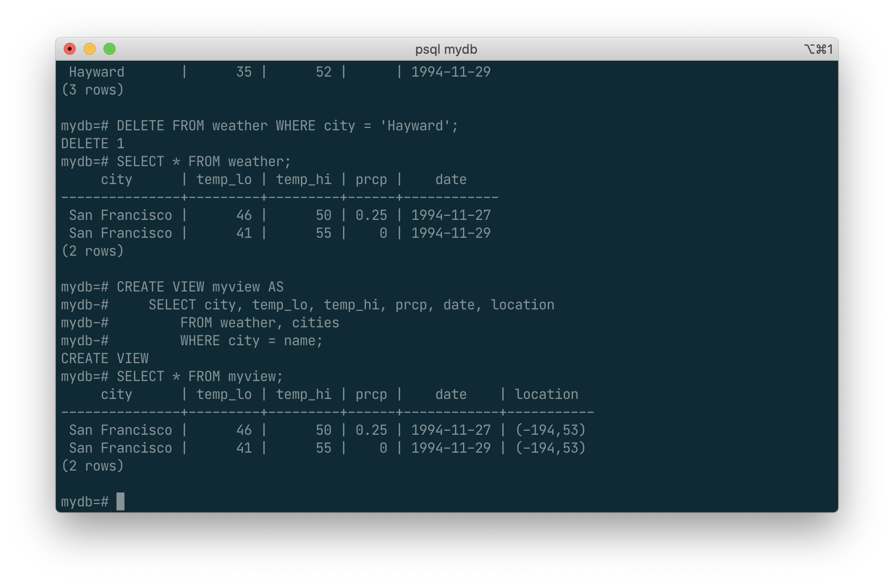
Deletions

Rows can be removed from a table using the DELETE command. Suppose you are no longer interested in the weather of Hayward. Then you can do the following to delete those rows from the table:

DELETE FROM weather WHERE city = 'Hayward';

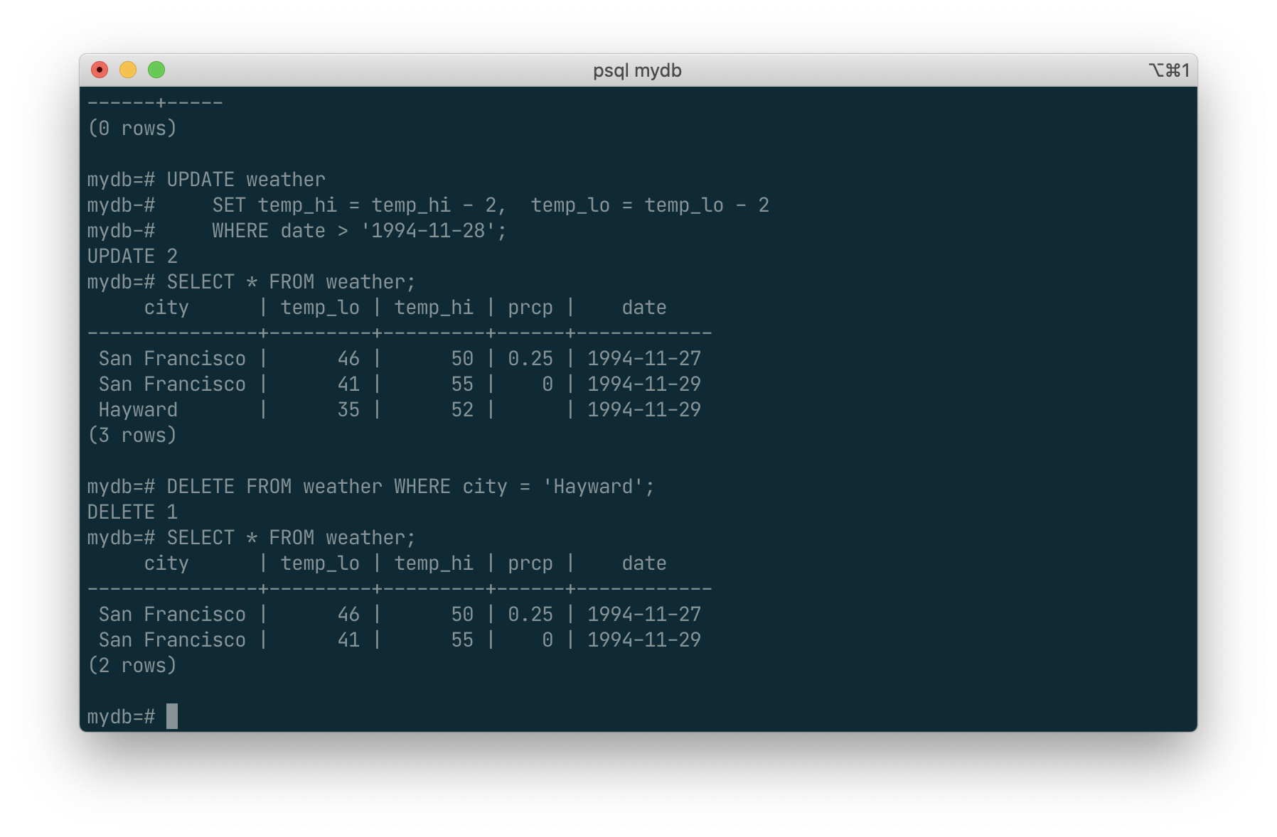
SQL Views

Suppose the combined listing of weather records and city location is of particular interest to your application, but you do not want to type the query each time you need it. You can create a view over the query, which gives a name to the query that you can refer to like an ordinary table:

CREATE VIEW myview AS
    SELECT city, temp_lo, temp_hi, prcp, date, location
        FROM weather, cities
        WHERE city = name;

SELECT * FROM myview;

Making liberal use of views is a key aspect of good SQL database design. Views allow you to encapsulate the details of the structure of your tables, which might change as your application evolves, behind consistent interfaces.

Foreign Keys

Recall the weather and cities tables from Chapter 2. Consider the following problem: You want to make sure that no one can insert rows in the weather table that do not have a matching entry in the cities table. This is called maintaining the referential integrity of your data. In simplistic database systems this would be implemented (if at all) by first looking at the cities table to check if a matching record exists, and then inserting or rejecting the new weather records. This approach has a number of problems and is very inconvenient, so PostgreSQL can do this for you.

The new declaration of the tables would look like this:

CREATE TABLE cities (
        city     varchar(80) primary key,
        location point
);

CREATE TABLE weather (
        city      varchar(80) references cities(city),
        temp_lo   int,
        temp_hi   int,
        prcp      real,
        date      date
);

TO do this, i’ve first deleted the myview using drop view myview; then deleted both tables : weather and cities using drop table table_name; way.

Now try inserting an invalid record:

INSERT INTO weather VALUES ('Berkeley', 45, 53, 0.0, '1994-11-28');

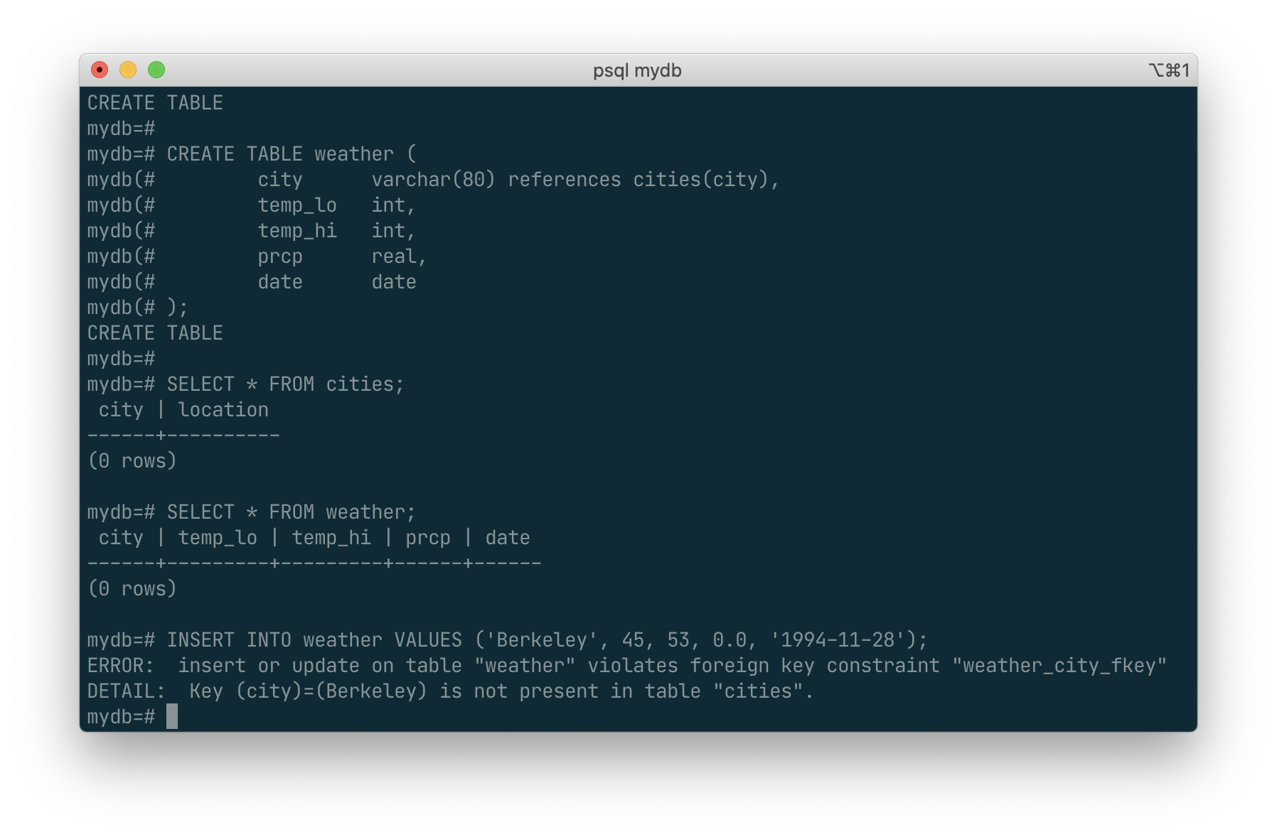
ERROR:  insert or update on table "weather" violates foreign key constraint "weather_city_fkey"
DETAIL:  Key (city)=(Berkeley) is not present in table "cities".

To make this happened, we should first create the city with the name, then create weather.

Transactions

Transactions are a fundamental concept of all database systems. The essential point of a transaction is that it bundles multiple steps into a single, all-or-nothing operation. The intermediate states between the steps are not visible to other concurrent transactions, and if some failure occurs that prevents the transaction from completing, then none of the steps affect the database at all.

For example, consider a bank database that contains balances for various customer accounts, as well as total deposit balances for branches. Suppose that we want to record a payment of $100.00 from Alice’s account to Bob’s account. Simplifying outrageously, the SQL commands for this might look like:

UPDATE accounts SET balance = balance - 100.00
    WHERE name = 'Alice';
UPDATE branches SET balance = balance - 100.00
    WHERE name = (SELECT branch_name FROM accounts WHERE name = 'Alice');
UPDATE accounts SET balance = balance + 100.00
    WHERE name = 'Bob';
UPDATE branches SET balance = balance + 100.00
    WHERE name = (SELECT branch_name FROM accounts WHERE name = 'Bob');

The details of these commands are not important here; the important point is that there are several separate updates involved to accomplish this rather simple operation. Our bank’s officers will want to be assured that either all these updates happen, or none of them happen. It would certainly not do for a system failure to result in Bob receiving $100.00 that was not debited from Alice. Nor would Alice long remain a happy customer if she was debited without Bob being credited. We need a guarantee that if something goes wrong partway through the operation, none of the steps executed so far will take effect. Grouping the updates into a transaction gives us this guarantee. A transaction is said to be atomic: from the point of view of other transactions, it either happens completely or not at all.

We also want a guarantee that once a transaction is completed and acknowledged by the database system, it has indeed been permanently recorded and won’t be lost even if a crash ensues shortly thereafter. For example, if we are recording a cash withdrawal by Bob, we do not want any chance that the debit to his account will disappear in a crash just after he walks out the bank door. A transactional database guarantees that all the updates made by a transaction are logged in permanent storage (i.e., on disk) before the transaction is reported complete.

Another important property of transactional databases is closely related to the notion of atomic updates: when multiple transactions are running concurrently, each one should not be able to see the incomplete changes made by others. For example, if one transaction is busy totalling all the branch balances, it would not do for it to include the debit from Alice’s branch but not the credit to Bob’s branch, nor vice versa. So transactions must be all-or-nothing not only in terms of their permanent effect on the database, but also in terms of their visibility as they happen. The updates made so far by an open transaction are invisible to other transactions until the transaction completes, whereupon all the updates become visible simultaneously.

In PostgreSQL, a transaction is set up by surrounding the SQL commands of the transaction with BEGIN and COMMIT commands. So our banking transaction would actually look like:

BEGIN;
UPDATE accounts SET balance = balance - 100.00
    WHERE name = 'Alice';
-- etc etc
COMMIT;

If, partway through the transaction, we decide we do not want to commit (perhaps we just noticed that Alice’s balance went negative), we can issue the command ROLLBACK instead of COMMIT, and all our updates so far will be canceled.

PostgreSQL actually treats every SQL statement as being executed within a transaction. If you do not issue a BEGIN command, then each individual statement has an implicit BEGIN and (if successful) COMMIT wrapped around it. A group of statements surrounded by BEGIN and COMMIT is sometimes called a transaction block.

It’s possible to control the statements in a transaction in a more granular fashion through the use of savepoints. Savepoints allow you to selectively discard parts of the transaction, while committing the rest. After defining a savepoint with SAVEPOINT, you can if needed roll back to the savepoint with ROLLBACK TO. All the transaction’s database changes between defining the savepoint and rolling back to it are discarded, but changes earlier than the savepoint are kept.

After rolling back to a savepoint, it continues to be defined, so you can roll back to it several times. Conversely, if you are sure you won’t need to roll back to a particular savepoint again, it can be released, so the system can free some resources. Keep in mind that either releasing or rolling back to a savepoint will automatically release all savepoints that were defined after it.

All this is happening within the transaction block, so none of it is visible to other database sessions. When and if you commit the transaction block, the committed actions become visible as a unit to other sessions, while the rolled-back actions never become visible at all.

Remembering the bank database, suppose we debit $100.00 from Alice’s account, and credit Bob’s account, only to find later that we should have credited Wally’s account. We could do it using savepoints like this:

BEGIN;
UPDATE accounts SET balance = balance - 100.00
    WHERE name = 'Alice';
SAVEPOINT my_savepoint;
UPDATE accounts SET balance = balance + 100.00
    WHERE name = 'Bob';
-- oops ... forget that and use Wally's account
ROLLBACK TO my_savepoint;
UPDATE accounts SET balance = balance + 100.00
    WHERE name = 'Wally';
COMMIT;

This example is, of course, oversimplified, but there’s a lot of control possible in a transaction block through the use of savepoints. Moreover, ROLLBACK TO is the only way to regain control of a transaction block that was put in aborted state by the system due to an error, short of rolling it back completely and starting again.

Window Functions

A window function performs a calculation across a set of table rows that are somehow related to the current row. This is comparable to the type of calculation that can be done with an aggregate function. However, window functions do not cause rows to become grouped into a single output row like non-window aggregate calls would. Instead, the rows retain their separate identities. Behind the scenes, the window function is able to access more than just the current row of the query result.

Here is an example that shows how to compare each employee’s salary with the average salary in his or her department:

SELECT depname, empno, salary, avg(salary) OVER (PARTITION BY depname) FROM empsalary;

depname  | empno | salary |          avg          
-----------+-------+--------+-----------------------
 develop   |    11 |   5200 | 5020.0000000000000000
 develop   |     7 |   4200 | 5020.0000000000000000
 develop   |     9 |   4500 | 5020.0000000000000000
 develop   |     8 |   6000 | 5020.0000000000000000
 develop   |    10 |   5200 | 5020.0000000000000000
 personnel |     5 |   3500 | 3700.0000000000000000
 personnel |     2 |   3900 | 3700.0000000000000000
 sales     |     3 |   4800 | 4866.6666666666666667
 sales     |     1 |   5000 | 4866.6666666666666667
 sales     |     4 |   4800 | 4866.6666666666666667
(10 rows)

The first three output columns come directly from the table empsalary, and there is one output row for each row in the table. The fourth column represents an average taken across all the table rows that have the same depname value as the current row. (This actually is the same function as the non-window avg aggregate, but the OVERclause causes it to be treated as a window function and computed across the window frame.)

A window function call always contains an OVER clause directly following the window function’s name and argument(s). This is what syntactically distinguishes it from a normal function or non-window aggregate. The OVER clause determines exactly how the rows of the query are split up for processing by the window function. The PARTITION BY clause within OVER divides the rows into groups, or partitions, that share the same values of the PARTITION BY expression(s). For each row, the window function is computed across the rows that fall into the same partition as the current row.

You can also control the order in which rows are processed by window functions using ORDER BY within OVER. (The window ORDER BY does not even have to match the order in which the rows are output.) Here is an example:

SELECT depname, empno, salary,
       rank() OVER (PARTITION BY depname ORDER BY salary DESC)
FROM empsalary;

depname  | empno | salary | rank 
-----------+-------+--------+------
 develop   |     8 |   6000 |    1
 develop   |    10 |   5200 |    2
 develop   |    11 |   5200 |    2
 develop   |     9 |   4500 |    4
 develop   |     7 |   4200 |    5
 personnel |     2 |   3900 |    1
 personnel |     5 |   3500 |    2
 sales     |     1 |   5000 |    1
 sales     |     4 |   4800 |    2
 sales     |     3 |   4800 |    2
(10 rows)

As shown here, the rank function produces a numerical rank for each distinct ORDER BY value in the current row’s partition, using the order defined by the ORDER BYclause. rank needs no explicit parameter, because its behavior is entirely determined by the OVER clause.

The rows considered by a window function are those of the “virtual table” produced by the query’s FROM clause as filtered by its WHERE, GROUP BY, and HAVING clauses if any. For example, a row removed because it does not meet the WHERE condition is not seen by any window function. A query can contain multiple window functions that slice up the data in different ways using different OVER clauses, but they all act on the same collection of rows defined by this virtual table.

We already saw that ORDER BY can be omitted if the ordering of rows is not important. It is also possible to omit PARTITION BY, in which case there is a single partition containing all rows.

There is another important concept associated with window functions: for each row, there is a set of rows within its partition called its window frame. Some window functions act only on the rows of the window frame, rather than of the whole partition. By default, if ORDER BY is supplied then the frame consists of all rows from the start of the partition up through the current row, plus any following rows that are equal to the current row according to the ORDER BY clause. When ORDER BY is omitted the default frame consists of all rows in the partition. [4] Here is an example using sum:

SELECT salary, sum(salary) OVER () FROM empsalary;

salary |  sum  
--------+-------
   5200 | 47100
   5000 | 47100
   3500 | 47100
   4800 | 47100
   3900 | 47100
   4200 | 47100
   4500 | 47100
   4800 | 47100
   6000 | 47100
   5200 | 47100
(10 rows)

SELECT salary, sum(salary) OVER (ORDER BY salary) FROM empsalary;

salary |  sum  
--------+-------
   3500 |  3500
   3900 |  7400
   4200 | 11600
   4500 | 16100
   4800 | 25700
   4800 | 25700
   5000 | 30700
   5200 | 41100
   5200 | 41100
   6000 | 47100
(10 rows)

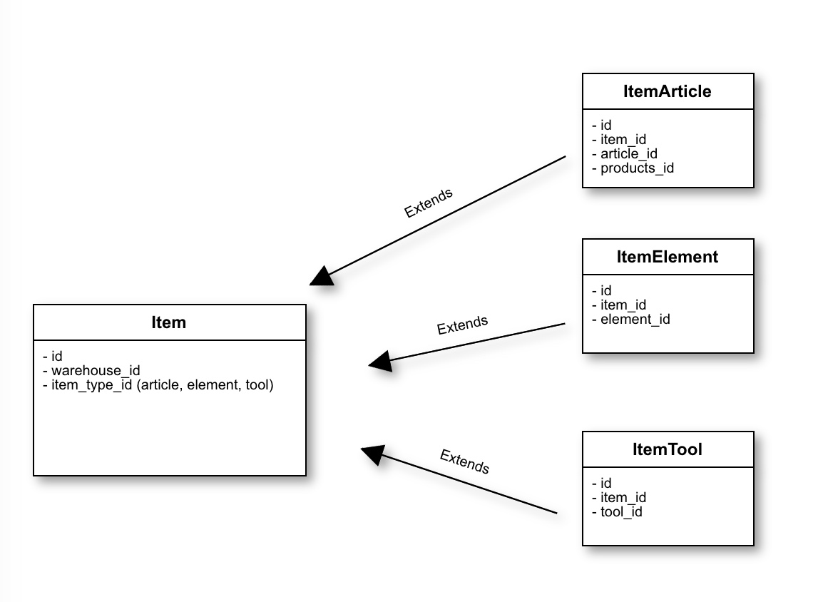
Inheritance

Inheritance is a concept from object-oriented databases. It opens up interesting new possibilities of database design.

Inheritance:

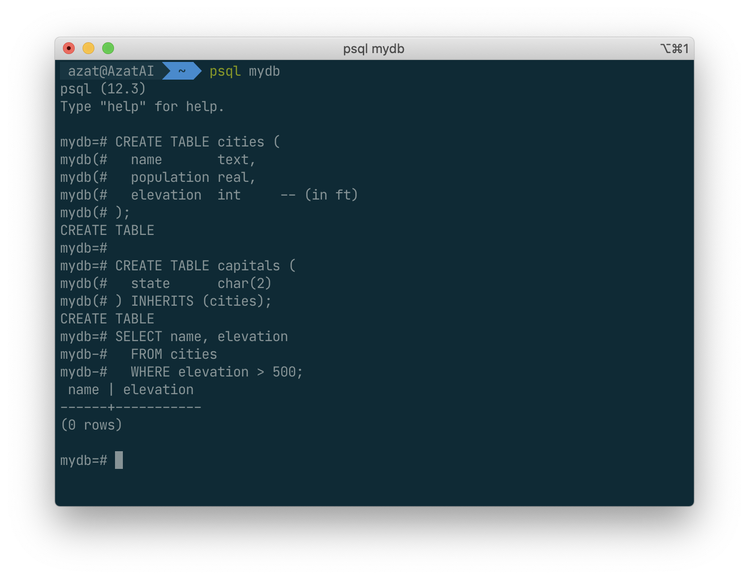
Let’s create two tables: A table cities and a table capitals. Naturally, capitals are also cities, so you want some way to show the capitals implicitly when you list all cities. If you’re really clever you might invent some scheme like this:

CREATE TABLE capitals (
  name       text,
  population real,
  elevation  int,    -- (in ft)
  state      char(2)
);

CREATE TABLE non_capitals (
  name       text,
  population real,
  elevation  int     -- (in ft)
);

CREATE VIEW cities AS
  SELECT name, population, elevation FROM capitals
    UNION
  SELECT name, population, elevation FROM non_capitals;

This works OK as far as querying goes, but it gets ugly when you need to update several rows, for one thing.

A better solution is this:

CREATE TABLE cities (
  name       text,
  population real,
  elevation  int     -- (in ft)
);
SELECT name, elevation
  FROM cities
  WHERE elevation > 500;
CREATE TABLE capitals (
  state      char(2)
) INHERITS (cities);

n this case, a row of capitals inherits all columns (name, population, and elevation) from its parent, cities. The type of the column name is text, a native PostgreSQL type for variable length character strings. State capitals have an extra column, state, that shows their state. In PostgreSQL, a table can inherit from zero or more other tables.

For example, the following query finds the names of all cities, including state capitals, that are located at an elevation over 500 feet:

SELECT name, elevation
  FROM cities
  WHERE elevation > 500;

On the other hand, the following query finds all the cities that are not state capitals and are situated at an elevation over 500 feet:

SELECT name, elevation
    FROM ONLY cities
    WHERE elevation > 500;

Here the ONLY before cities indicates that the query should be run over only the cities table, and not tables below cities in the inheritance hierarchy. Many of the commands that we have already discussed — SELECT, UPDATE, and DELETE — support this ONLY notation.

Advances SQL Language

TO BE CONTINUED.