Trading with AI

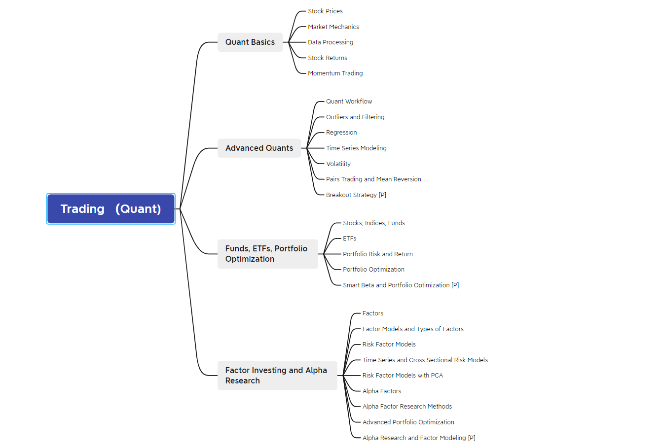
Quant Basics

Stock Prices

Stocks

You’ve probably heard of stocks ¹and shares² before. Shares of stock represent fractional ownership in a company. If you own one share of a company stock and the stock has been split into eight shares in total or eight shares outstanding, you own one-eighth of the company.

There are actually two types of stock : common and preferred stock.

Stock:

1. common stock ³

   • Shareholders who own common stock usually get a portion of the company’s profits in the form of dividends⁴ if the company distributes them.

   Note ： A dividend is a payment made by a corporation to its investors, usually as a distribution of profits.

   • Shareholders also get the right to vote
   • If the company is liquidated due to bankruptcy, they also get a portion of the remaining assets after all other stakeholders are compensated⁵.

2. preferred stock ⁶

   • Shareholders who own preferred stock get a slightly different deal, they’re promised a fixed amount of income each year and get paid before owners of common stock get paid dividends, but they usually do not have voting rights.

But of course, one of the main benefits of owning stock is the potential opportunity to profit from selling it after it’s value has increased. These increases in value are called capital gains ⁷.

We’re primarily referring to common stock as opposed to preferred stock. This is because preferred stock actually behaves more like a bond⁸ (which we’ll cover next), so preferred stock prices may tend to be more stable relative to common stock of the same company. Usually when you see stock data and financial news, it’s referring to common stock.

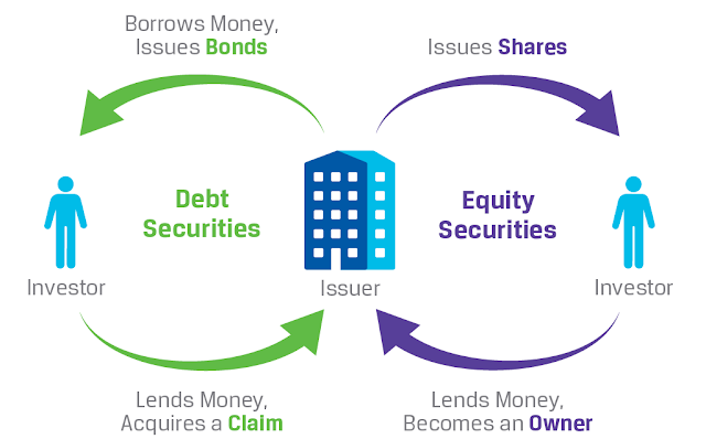
• A security⁹ is a financial instrument that has some type of monetary value¹⁰.
• Securities can be classified into three broad types;
• 

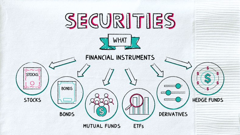
graph LR
A[security]-->B[Debt Securities]
A-->C[Derivative Securities]
A-->D[Equity Securities]

B-->E[Bonds]
B-->F[Certificate of Deposit]

C-->G[Options]
C-->H[Future Contracts]

• Debt Security¹¹:
  • represent money that is owed and must be repaid¹².
  • government or corporate bonds¹³
  • certificates of deposit¹⁴
  • Debt securities are also called fixed-income securities because they promise a stream of income over time in the form of interest¹⁵ either at a fixed rate or at a rate determined by a specific formula.

• Derivative Security¹⁶:

  

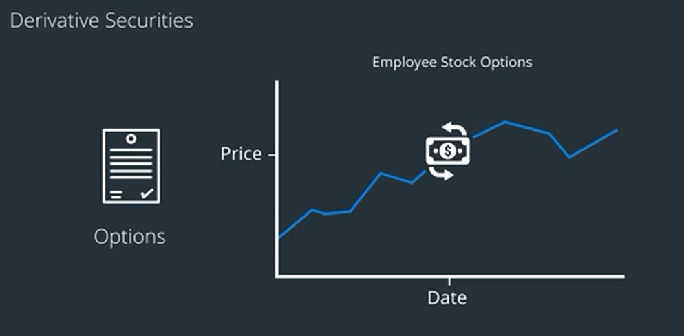
  • options ¹⁷
    • an option is a contract which gives the buyer the right but not the obligation¹⁸ to buy or sell an underlying asset at a specified price on a specified date.
  • futures contracts¹⁹
    • a futures contract obligates the buyer to buy or the seller to sell an asset at a predetermined price at a specified time in the future.
  • their values depend on the prices of other assets.

• Equity Securities²⁰:

  • Equity — Equity²¹ is the value of an owned asset minus the amount of all debts or liabilities²² on that asset.

  

  • The word equity can have somewhat different meanings in different contexts.

  • in general, you can think of equity as the net value of something owned.

  • Stocks are called equity securities because they represent ownership in a firm.

  • private equity — a security representing ownership interest in a private company

    

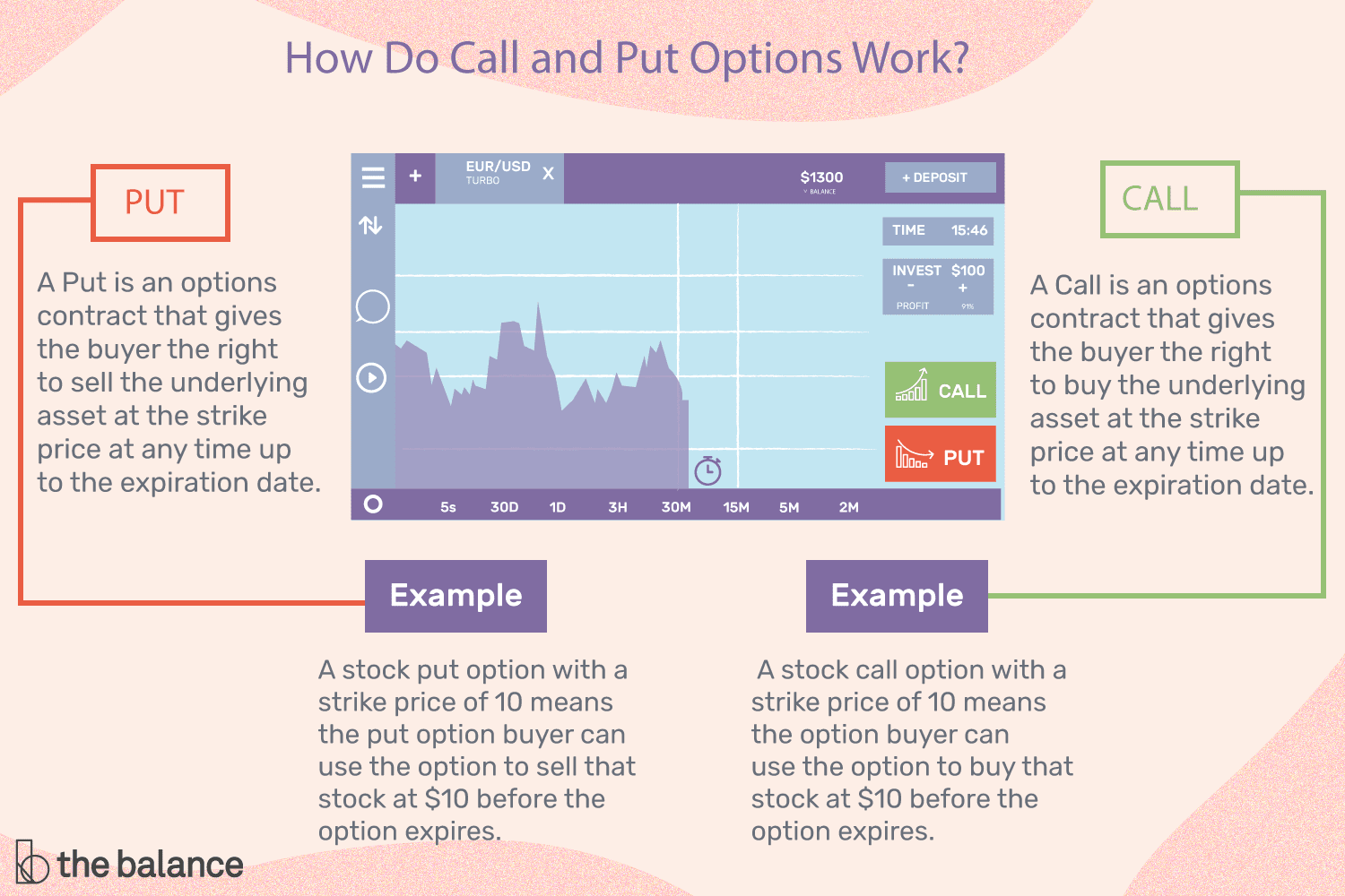
  Options: calls, puts, American, European

  Options give the owner the right to buy or sell at the strike price (a fixed price that is determined when the option is created), on or before an expiration date. The most common are call options and put options. Call options give the right to buy at the strike price; put options give the owner the right to sell at a fixed price. Some options allow the holder to “exercise” (buy or sell) at the strike price any time up to the expiration date. These are called “American options” by convention, even though this doesn’t mean that the options are traded in the Americas. Another class of options only allows the holder to exercise the option at the expiration date, but not earlier. These are called “European options” by convention, but again, European options don’t necessarily have to be traded in Europe.

  

  Forwards and Futures

  Futures and forwards contracts are similar, in that a buyer and seller both agree to make a future transaction at a predetermined price. Futures are standardized contracts that can be traded on a futures exchange, so this may be what people think of when discussing “forwards and futures”. Forward contracts are usually privately determined contracts between two parties. So an investor can trade futures contracts, but forward contracts are not designed to be traded like futures.

  Public versus private equity

  Public equity refers to stocks that can be traded on a stock exchange. Private equity refers to ownership in private companies, so the owners of private equity do not trade their shares on a stock exchange.

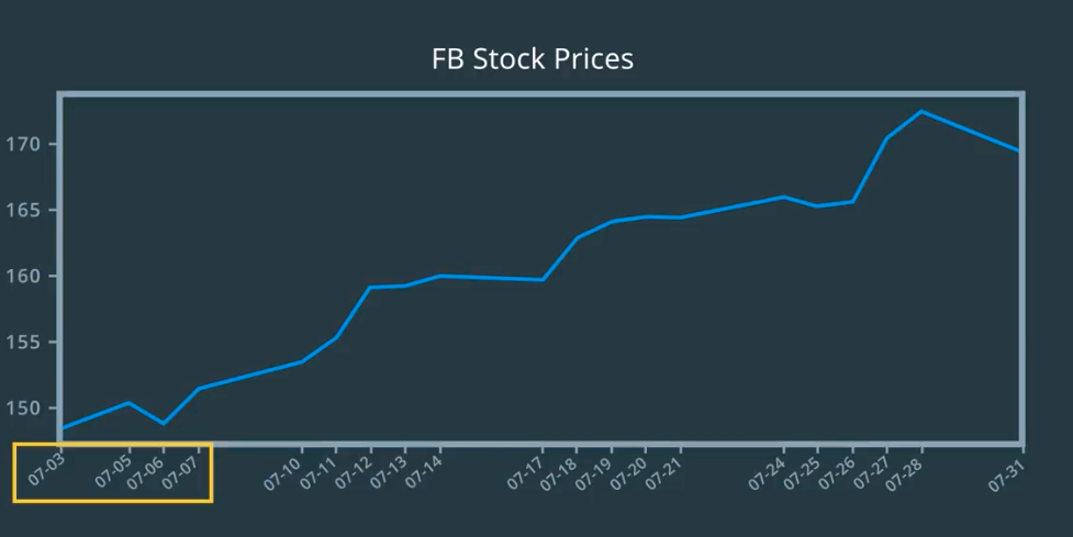
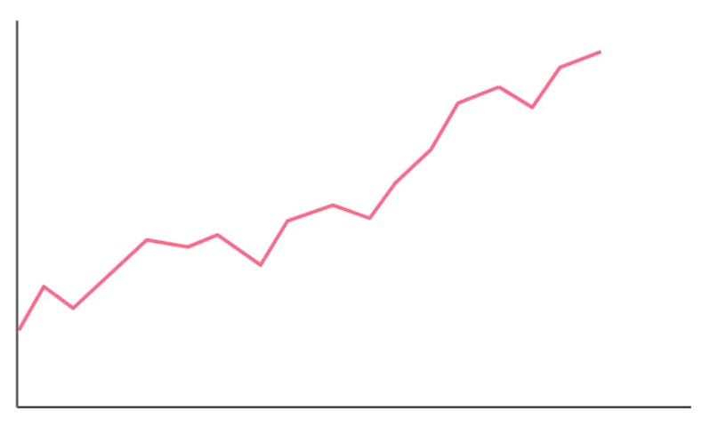
Stock Prices

• Brokerage²³ :
  • A brokerage company functions as a middleman connecting buyers and sellers.
  • they usually charge fees to complete transactions.
• in order to make money from your investment :
  • sell it when its price is higher than when you bought it.
  • predicting when the price of a stock will go up.
• unique symbol or ticker²⁴
  • Alphabets unique symbol is GOOG
  • Apples ticker is AAPL
• The history of a stock’s price is important
  • potentially an indicator of how the stock will do in the future.
• One of the most interesting market phenomena is the market bubble.
  • Bubbles occur when market participants drive stock prices above their value in relation to some system evaluation.
• Extra：
  • Robert Shiller
  • Nassim Taleb
• Further resources
  • Robert Shiller’s home page
  • Robert Shiller’s “Economic View” column for the New York Times
  • Nassim Taleb’s home page
  • Nassim Taleb lecture, “How do you solve a problem like uncertainty?”
  • Nassim Taleb op-ed, “Stabilization won’t save us.”

Terminology

Stock : An asset²⁵ that represents ownership in a company. A claim on part of a corportation’s assets and earnings. There are two main types, common and preferred .

Share : A single share represents partial ownership of a company relative to the total number of shares in existence.

Common Stock : One main type of stock; entitles the owner to receive dividends and to vote at shareholder meetings.

Preferred Stock : The other main type of stock; generally does not entail voting rights, but entitles the owner to a higher claim on the assets and earnings of a company.

Dividend : A partial distribution of a company’s profits to shareholders.

Capital Gains : Profits that result from the sale of an asset at a price higher than the purchase price.

Security : A tradable financial asset.

Debt Security : Money that is owed and must be repaid, like government or corporate bonds, or certificates of deposit. Also called fixed-income securities.

Derivative Security : A financial instrument whereby its value is derived from other assets.

Equity : The value of an owned asset minus the amount of all debts on that asset.

Equity Security : A security that represents fractional ownership in an entity, such as stock.

Option Contract : A contract which gives the buyer the right, but not the obligation, to buy or sell an underlying asset at a specified price on or by a specified date

Futures Contract : A contract that obligates the buyer to buy or the seller to sell an asset at a predetermined price at a specified time in the future

Market Mechanics

First build a simple market simulator that matches and executes orders, and sets prices just like a real market. This will give you a better idea of all the activities that keep a market running. These activities generate a lot of data.

Market data, which may hold important clues that you can use to decide when to buy or sell stocks. As you get introduced to the various dimensions of data available to us, try to build an intuition for why they might be important, what signals they might carry.

Finally, you will learn to deal with data during the closing and opening of global markets. If you pay close attention, there might be some training opportunities there too.

Trading Stocks

When a company first begins trading publicly it typically picks a value for its stock based on certain company metrics like revenue²⁶, profits²⁷, assets et cetera. But from that point on, it’s stock prices almost entirely driven by how much demand exists for its stock.

Modern markets keep an electronic record of all orders that have been submitted.

• People who want to buy a stock can specify how much or the limit that they’re willing to pay for it.

• People who want to sell can specify the least amount. Again the limit they’re willing to sell it for.
• Whenever a suitable match is found between a buyer and seller, a trade is executed.

The stock exchange keeps track of the last price at which a stock was traded. This is publicly posted as the current price of the stock, and if you wish to buy or sell shares around that price you should be able to do that immediately. This is known as placing a market order.

But it does introduce one complication, someone has to be willing to sell or buy that stock on the other end at all times. That’s where a market maker comes into the picture.

• A market maker²⁸ is a financial firm. Usually a brokerage that continuously offers to buy and sell stocks at publicly advertised prices.

There are buyers and sellers who go through the stock exchange to buy a stock that they think will do well, or sell a stock that they wish to remove from their investments.

Market maker serves as the counterparty²⁹ of these buyers or sellers. Since every buyer needs a seller, and every seller needs a buyer, a market maker plays the role of seller to those who wish to buy, and plays the role of buyer for those who wish to sell.

By convention³⁰, we refer to these market makers as the “sell side” of the finance industry. The sell side includes investment banks such as Goldman Sachs and Morgan Stanley. The buy side refers to individual investors, and investment funds such as mutual funds³¹ and hedge funds.

Liquidity

Imagine what would happen without market-makers? It would be harder to buy or sell stocks at a consistent price. As people start selling a stock, its price would start falling and vice versa.

Formally, we say that a market maker provides liquidity³². Liquidity is the property of a financial asset like a stock, to be bought or sold without causing sharp changes in its price.

On the other hand, stocks that are relatively difficult to buy or sell are said to be illiquid ³³.

Penny stocks³⁴, for example, are typically very thinly traded. Consequently, buying or selling them may be difficult.

Liquidity can also vary from market to market. The same stock can be bought or sold in different markets. Each market maintains its own book of orders so the same stock can trade at different prices in different markets. The difference is usually small, and any big changes permeate across markets pretty quickly.

That being said, it’s possible to profit from market inefficiencies by simultaneously purchasing and selling an asset in different markets, thereby exploiting the differences in price. This idea is known as arbitrage³⁵.

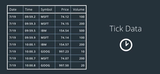
Tick Data

Stock exchanges³⁶ publish a stream of data that includes each individual trade. This is known as tick data. Ticks are an intuitive³⁷ way to gauge³⁸ the health of a stock or even an entire market.

For example, you can compare each stock’s latest tick price with its previous price to see if it is going up or down. You can then aggregate³⁹ this information by comparing the number of stocks on an up-tick with the number of stocks on a down-tick.

These ticks also form the basis for all market data that is available for analysis. Tick data can provide further insight into how a particular stock is behaving and can help you take better intraday decisions, but you’re talking about a massive volume of data.

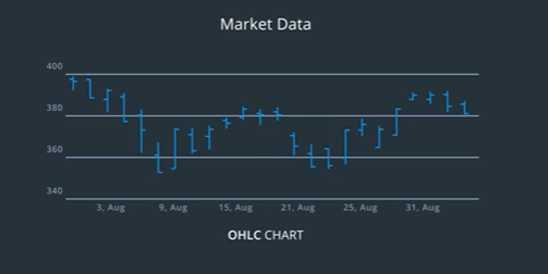
OHLC: Open, High, Low, Close

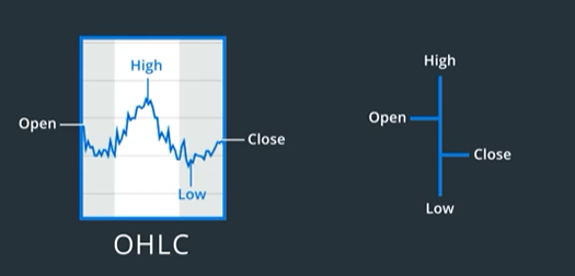
The most common set of measures used in practice are Open High Low Close or OHLC. Open is the stock price at the beginning of the period, high and low capture its range of movement, and close is where it ends.

These measures are often visualized using OHLC bars, which show these four measures for each time interval in a compact form.

The daily closing price is the one that is coded most often. It is used by casual traders and investors who are interested in long-term gains. It is also used for accounting purposes. The opening price, is where you would expect the first trade of the day to take place. There might be a gap from last day’s closing price, because of pre-market trading or trading in other markets.

Volume

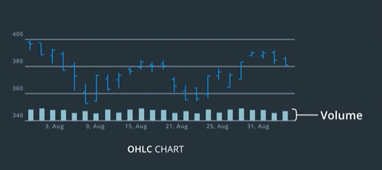
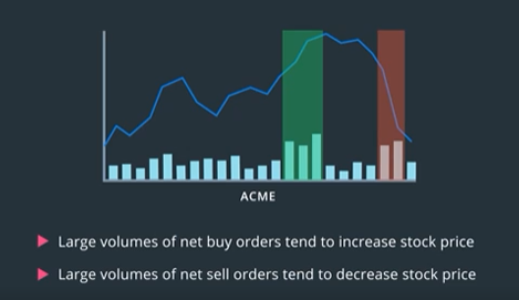
Besides the current price of a particular stock. Another metric that traders liked to keep an eye on is the number of shares that are being traded over a period of time known as volume. Often shown along the bottom of an OHLC chart.

The sum of unit price times volume gives you a more accurate measure of the total amount of money moving around.

Volume is also important because it can affect how sharply its price might rise or fall.

In general, large volumes of buy orders tend to sharply increase the stock price and large volumes of sell orders make it fall. This is another signal that you can use to decide when to trade a given stock.

Note that the volume of transactions also varies throughout any trading day. This is something to be aware of if you want to use volume as a trading signal. Stocks that are of active interest will typically see a lot of training at the beginning of the day. Since that is when traders get to act on, all the new information gathered and analyzed since the previous day’s market close. This initial activity known as price discovery, helps buyers and sellers converge on a mutually acceptable market price for each stock. Then the volume falls to a lower level as typical daily trading activity resumes. Finally, towards the end of the trading day, activity tends to increase a little resulting in a higher volume. This can be due to several reasons including day traders who want to close out any open positions and funds that typically update their holdings at the end of the day.

In fact, some traders who have decided to buy-sell particular stocks, may not want to risk waiting for the next day.

Gaps In Market Data

Stock markets typically remain open for a finite number of hours every day, say 9:30 AM to 4:00 PM. This is when the majority of the transactions take place.

With the growing popularity of algorithmic trading, a large portion of transactions today are being carried out by automated systems. They can be much more responsive to market conditions than humans, and result in a sharp increase or decrease in stock prices over a very short period of time. If left unchecked, this can result in things spiraling out of control. Closing market operations at a regular time every day provides an artificial barrier that can limit the damage such events can cause. This also give stock market regulators some time to analyze the situation and implement control measures.

Stock markets close operations at a certain time every day, and they typically remain closed over weekends and holidays. As a result, when you look at stock data, you’ll notice these gaps or discontinuities during periods when the markets are closed.

Depending on your analysis, this may or may not have an impact on the conclusions you draw.

For instance, if you treat market data as a simple sequence of observations and ignore the timestamps as if the market’s just smoothly continue from one end of day to the next opening bell, then these gaps are not as significant.

But, if you compute a metric that involves time like the number of transactions per hour, then ignoring these gaps can give you inaccurate results. The discontinuities can produce spikes or unusual flats in calculated values, or just outright wrong information. So, you need to be careful when dealing with market data.

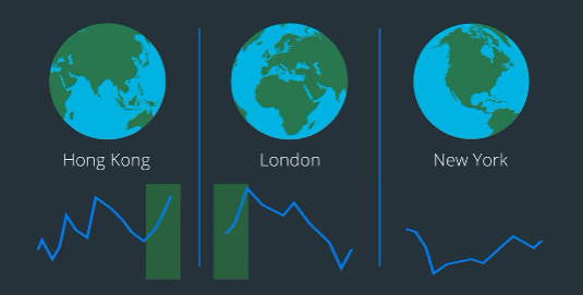
Markets in Different Time zones

Another aspect worth considering is that most major stock markets are actual physical buildings located in a city somewhere on the planet, and because different cities around the globe are at different time zones, the actual opening and closing times also vary.

The Hong Kong Stock Exchange opens at 09:30 AM local time.

London Stock Exchange opens at 09:30 AM their local time.

New York Stock Exchange opens five hours after that.

This produces some additional complications and opportunities for traders. For example, consider the stocks that are listed on multiple global exchanges.

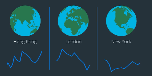
If HSBC rises in Hong Kong, you can buy HSBC in London the moment the market opens, knowing that it is likely to rise there too. Of course, you have to be careful about how you execute such strategies. Remember that if you are trying to take advantage of markets in different time zones, chances are high that other traders are too.

Note on ADR : Foreign stocks are sometimes allowed to trade on a local stock exchange via an indirect method such as American Depository Receipts (ADR). These are instruments that represent the original stock in a different market.

Data Processing

Market Data

The data is the most important thing to quantitative analysis. Without good data, you don’t have good predictions. That is sometimes referred to as the garbage in, garbage out principle. That is the quality of your data directly impacts the quality of your predictions, no matter what model you use.

Note : Tick data is sometimes referred to as heterogeneous⁴⁰ data, since it is not sampled at regular time intervals, whereas Minute-level or End-of-Day data is called homogeneous⁴¹.

This is any data that you receive from the market typically generated from trades. This is perhaps the most important form of data relevant to quantitative analysis. it’s a series of trading events that happen in a moment of time, each moment is called a tick.

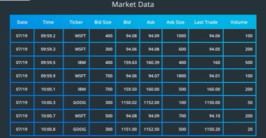
A ticker contains the time of the event, information about which stock or ticker symbol is traded trade data and quote data.

The trade data is the price and the amount of the transaction.

The quote data is the price and size of the bid and ask.

A bid is request to buy stock at a price for a set amount of shares.

A ask is the other side of the trade it’s the request to sell stock at a price for a set amount of shares.

In large marketplaces the number of trades can easily hit 200 trades per second. This is a massive amount of data when using historical tech data. Analyzing individual texts may not be visible with this much data.

So, we bucket these texts into equally space time integrals such as minutes or days. For each bucket, we can compute open high low close prices and total volume of transactions. This sort of minute or day level data is much easier to work with.

You have the ability to ignore the timestamps and treat the data as equally spaced sequences.

Note: In some cases, you may still need to use the timestamps.

Corporate Actions: Stock Splits

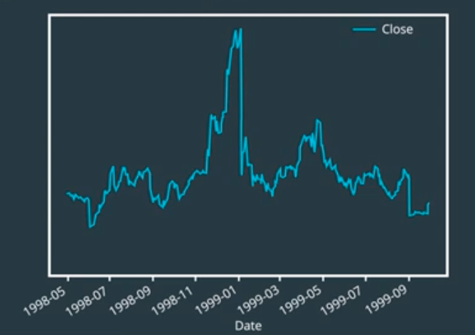
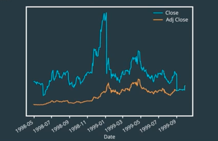
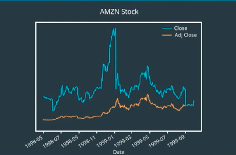
On June 2nd, 1998, you could buy a share of Amazon for about $85. On this date, Amazon decided to perform a two to one stock split. Every Amazon shareholder, had their shares doubled. This does not mean all of their money in Amazon doubled. When a stock is split into two, its price drops by half.

This makes sure that the total market capitalization of a stock has not changed by a split. Market capitalization is the dollar value of a company’s outstanding shares. This is calculated by multiplying the stock price by the total number of shares outstanding.

Why would you ever want to split a stock? One reason could be to make the stock more liquid.

Using these prices, a computer would read the data the same way. However, this is not true. The value of the company has not changed from the split. How do you correct for this? One common approach is to normalize the prices to reduce the sudden changes.

We’ll have the price before each two-to-one split, turn it into thirds before any three-to-one split, and so on.

Now, the newest adjusted price matches the price currently on the market. Stock prices normalized in this manner is called adjusted price. This is typically provided in most historical data sets.

Corporate Actions: Dividens

Dividends are when companies share some fraction of their profits with their shareholders. Whoever held the stock before the state will receive the dividend. With the basics of dividends out of the way, let’s go over adjusting the prices to dividends.

We’ll start with why we adjust the prices based on dividends. Imagine that you own one share of company A and one share of company B, both are worth $50.

The next day is an ex-dividend date of $1 in dividends for company A.

That day, company A closes at 49.50. Company B does not have ex-dividend date, but also closes at $49.50.

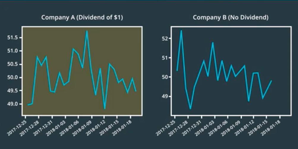
If you only looked at the prices, you might think you lost $0.50 on both stocks. In reality, you made $0.50 on company A and lost $0.50 on company B.

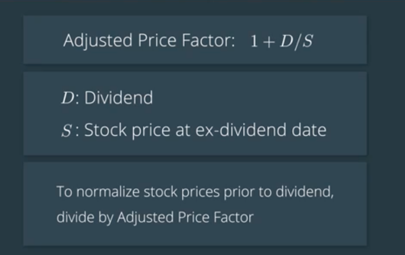
Just like the stock splits, we’ll normalize the prices to reflect this. To get the normalised prices, we first need to calculate the adjusted price factor. The formula for this is 1+D over S. D is the dividend, S is the stock price at ex-dividend date. To normalize the price, you would divide the historical price by the adjusted price factor up until the day before the ex-dividend date.

Aside : Although a stock split shouldn’t theoretically affect the market cap of a stock, in reality it does! There are some intriguing⁴² behavioral patterns that researchers have observed among traders. One seems to suggest that after a stock splits, and the price drops considerably, people seem to think it is going to go back up to the previous price (double or triple)! This creates an artificial demand for the stock, which in turn actually pushes up the price.

Technical Indicators

So, you have your stock prices adjusted for corporate actions like splits and dividends. How do you use this information to perform trading? When you buy, when you sell, or even which stocks do you buy or sell.

• when to buy
• when to sell
• which to buy OR sell

You can take these decisions based on signals that can be derived⁴³ from historical price data. The first step in this process is to compute statistical measures that are called indicators. You can think of the raw price of a stock as the most basic kind of indicator.

The price seems to be jumping around a lot and we don’t have a sense of where we should expect to be. If we had that, then we could check if their current price is significantly higher or lower than the expected price and make a decision based on that.

So, what is the expected price of a stock? Is it the average price from when it began trading? That seems a little too extreme. Stocks can grow in orders of magnitude over the years. Most current prices will be well over the average. What might be relevant is the recent average price of the stock. Maybe over the past week or month, we can extend this idea throughout the history of the stock and compute the average of a fixed length window of time.

It’s like moving the window one unit at a time and taking the average price within that window.

This is known as the simple moving average or rolling mean.

We could devise a trading strategy that looks for large deviations from the moving average, and generate trading signals based on that.

For instance, if a stock falls too far below its average, then we should buy it, or if it rises too far above, then we should sell.

But, how much is too much.

Using a constant number or a threshold does not seem like a good idea. Different stocks trade at different price levels.

We need a measure that is tied to the price of the stock, maybe some fraction of the stock price.

But again, what fraction? We don’t know.

Some stocks jump around a lot. Some are more stable. A better idea might be to compute the threshold from the jumpiness⁴⁴ or volatility⁴⁵ of the stock.

How about standard deviation⁴⁶?

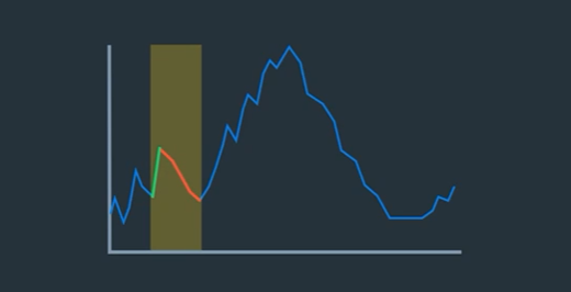
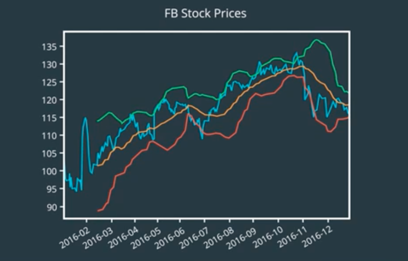
In fact, we can reuse the windowing idea and compute standard deviation over the same fixed length window across time. These lines are called Bollinger bands.

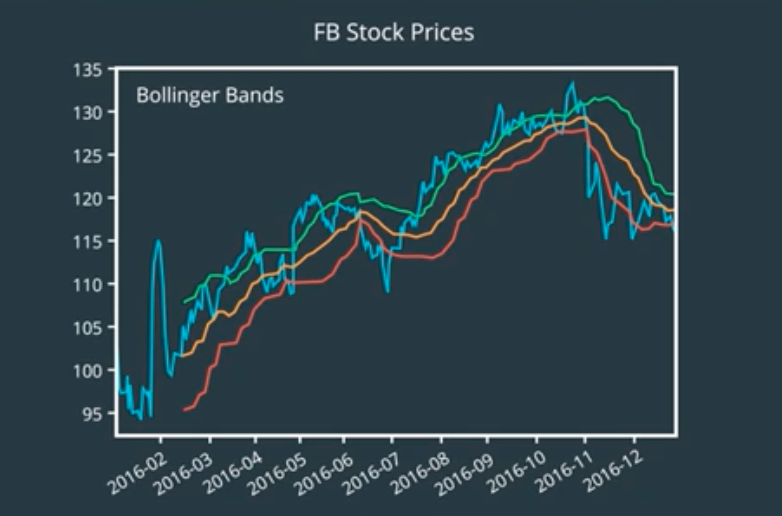
All these peaks sticking above the upper band are signaling that the stock is trading at a higher price than normal. The dips below the lower band are signaling abnormally low price.

One problem that you might notice is that there’s too many such points. We can reduce them by increasing the width of the bands. That is, by considering a wider range of variation to be normal. A common threshold is to choose two standard deviations above and below. Now, we have far fewer outliers⁴⁷.

But the question remains what do we do with these outlying points? Sometimes we get short burst of outliers.

So, should we buy or sell each of these points? If you think about it, when the price falls below the lower band, you don’t really know if it’s going to keep falling or is it going to rise back up.

Maybe it’s wiser to focus on these inflection points⁴⁸.

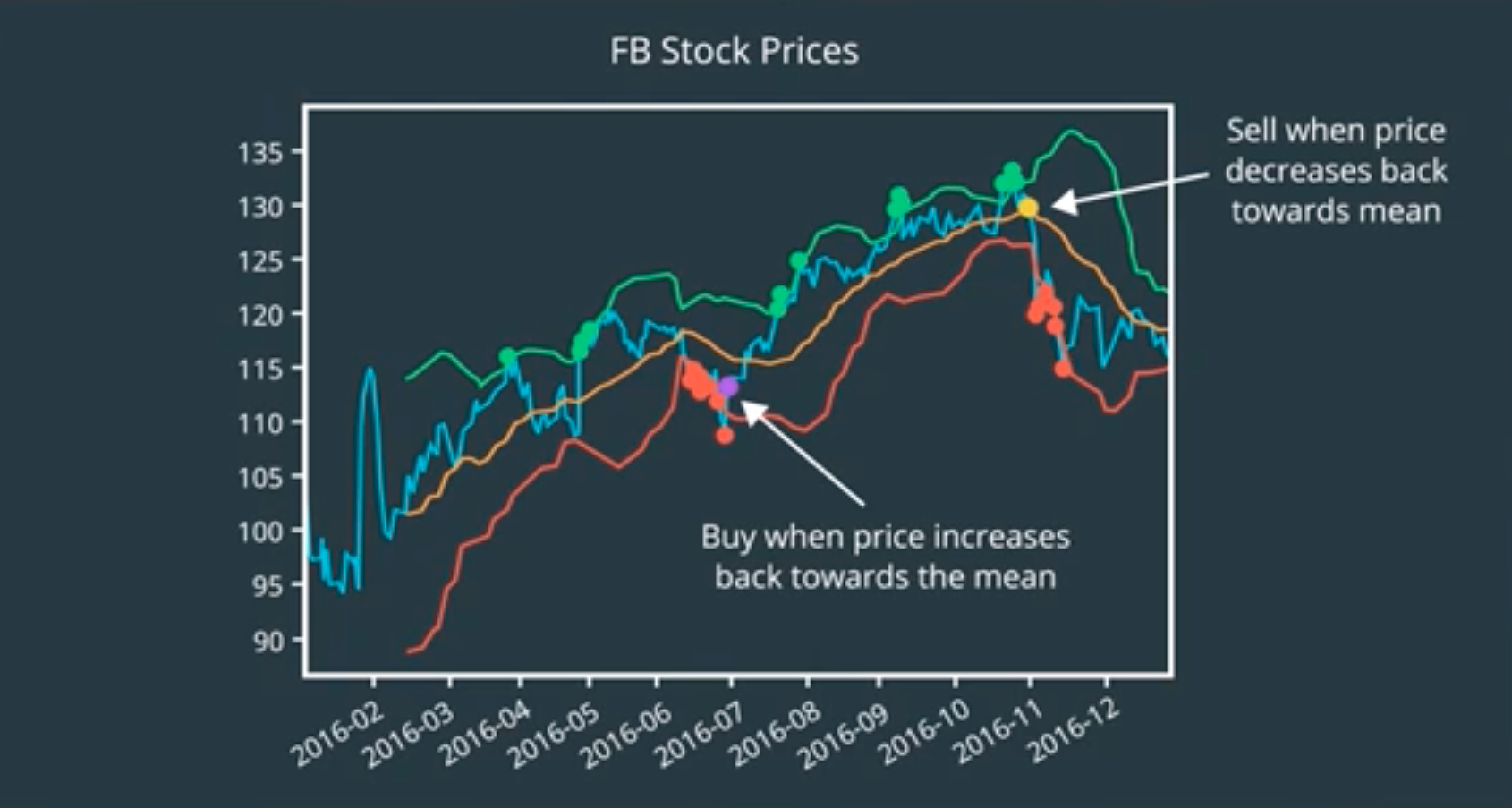
When the price is below the lower band and starts to cross back inside towards the mean, that should be a good time to buy.⁴⁹

The price is still fairly low and on a rise.

On the other side, we can sell when the price crosses down the upper band to the inside. ⁵⁰

This gives us a series of buy and sell signals.

Note : Moving-window or “rolling” statistics are typically calculated with respect to a past period. Therefore, you won’t have a valid value at the beginning of the resulting time series, till you have one complete period. For instance, when you compute the Simple Moving Average with a 1-month or 30-day window, the result is undefined for the first 29 days. This is okay, and smart data analysis libraries like Pandas will mark these with a special “NA” or “nan” value (not zero, because that would be indiscernible from an actual zero value!). Subsequent processing or plotting will interpret those as missing data points.

Missing Values

Up until now, we’ve been treating stock prices as a continuous time series. For instance, the end of day data for stock includes a row for every day or does it?

Gaps in the data can result from weekends, holidays, and other reasons the market might be closed. You might be thinking why is this important? After all, if we forget about these missing days, the data is still continuous in terms of trading days.

Well, that’s true if you treat the price data as simple sequence and ignore the timestamps, then you don’t need to worry about the gaps.

Say, you’re computing daily returns. Take the price on each day and subtract it from the price on the previous day. Well, previous trading day that is. For more robust approach to trading, you may not want to ignore the missing days. Even if the market is closed, other events can occur that might influence stock prices when the market reopens.

For example, company announcements, news articles, geopolitical events, natural disasters, anything and everything can affect the stock price.

The more time between two trading days, the bigger the window for things to happen.

Another kind of gap you should be aware of is the time between the market closes for the day and when it reopens the next day.

When a particular market opens for trading, the price of that stock can be different from the closing price on that market from the previous day.

Fundamental Information

Fundamental Analysis

Fundamental analysis of a company involves looking at a company’s balance sheet⁵¹ and cash flow statements, which are usually updated every quarter, which is every three months when the company reports earnings. It’s important to keep in mind that looking at a single quarter’s metrics is only a snapshot of the company, and there are several metrics that each try to capture the health of the company, but in slightly different ways.

Sales per Share

A company’s revenue⁵² is based on its sales over that quarter, so we can think of sales and revenue as referring to the same thing. It’s a quick way to get a sense for how a company is doing, because we don’t have to subtract out cost of sales, which depends a bit on some accounting decisions. For example, if a company sells a million smartphones for a hundred dollars each over the past 3 months, then its revenue is $100 times 1 million, or $100 million. If the company issued ten million shares, then its sales per share is $100 million divided by ten million, or $10 per share.

You may be wondering why we bother dividing sales by the number of shares. This helps shareholders get a sense of how much the sales figures might impact a change in a single share price. You can imagine that if the company only issued 10 shares, a report of higher sales than forecasted would impact each share more than if the company issued ten million shares.

Also, note that sales of $10 per share probably does not mean that the shareholders will get $10 for each share that they own, or that their stock price will increase by $10. It costs money for the company to make each smartphone. Let’s take a look at a metric that accounts for cost of sales next.

Earnings Per Share

Earnings is the company’s revenue minus its cost of sales. Cost of sales refers to the cost of manufacturing the phone, employee wages, rent payments for office space, and the cost of equipment, like machines that make the phones. Earnings gives investors a sense of how much the equity of the company has changed over the past 3 months. Recall that stock represents a fractional ownership of a company’s equity.

Continuing with the smartphone company example, let’s say we can estimate the cost of sales per phone to be $80 per phone. If the sales per phone is $100, then the earnings per phone is $100 - $80 equals $20 per phone. With sales of one million phones, earnings would be $20 times one million, or $20 million.

With ten million shares, this is earnings of $20 million divided by ten million shares, which is $2 earnings per share.

Note again, that this $2 per share doesn’t mean that investors automatically receive an additional $2 per share in their pocket. Let’s look at one way that investors do receive some of those earnings by looking at dividends.

Dividens Per Share

After a company has positive earnings, they may decide to either reinvest the cash in growing the company’s business. A company’s executives are usually expected to make spending decisions based on maximizing shareholder value. Whether this always happens in practice is debatable, but ideally, if the executives decide that re-investing in the business yields lower returns than an investor could gain from investing in a similar business at the same level of risk, they will give some of the earnings to shareholders as cash. This cash is referred to as dividends.

Let’s say, for example, that the smartphone company decides to return $10 million of its earnings to its shareholders. The dividend per share is then $10 million divided by 10 million, or $1 per share.

Price Earnings Ration

A term you’ll see often is price to earnings ratio, or PE ratio for short. This is the stock’s current market price divided by its most recently reported earnings per share (EPS). You can sort of interpret the PE ratio as how much the company is valued compared to how much money it made.

It’s important to be careful about how we interpret a high or low PE ratio, because we can’t say whether a PE ratio is good or bad by looking at it in isolation. Let’s first look at where the price comes from.

Now coming back to the PE ratio. What does it mean to have a high PE ratio? A company may have low or negative earnings, but a high stock price. Why do you think that is? You may have heard of certain startups that are valued at billions of dollars, and yet have low earnings. This is because investors expect potential for high earnings growth, based on the trajectory of past earnings growth. This also means that investors are estimating that the high stock price relative to earnings will be justified by high future earnings. On the other hand, it’s also possible that investor optimism towards the company’s future never materializes, in which case the stock may be overpriced.

Exchange Traded Funds (ETFs)

Let’s take a moment to think about what a trading algorithms goal should be. The obvious part is making money i.e, we should try to generate as much positive returns from trading as possible but the stock market is inherently very unpredictable as we have already seen.

One approach is to buy stocks that have been showing consistent growth and hold onto them for long periods of time.

This usually generates some returns but nothing spectacular⁵³ unless you happen to pick stocks that grow spectacularly.

But, how you tell ahead of time? What if they don’t do as well or even fall? This inherent risk in the market is very real. It is as much part of the game as the actual stock prices. To mitigate⁵⁴ this risk, you should maintain a fairly broad portfolio stocks instead of investing a handful⁵⁵.

How you choose these stocks can affect how much your returns are affected by market behavior.

So, how do you go about picking your basket of stocks? You could perform complex statistical analysis to find collections that are likely to generate good returns but also reduce the overall risk.

If you’re just investing your personal money, this might be too much work. Not everyone who wants to invest they have he knowledge and skills to conduct a proper analysis.

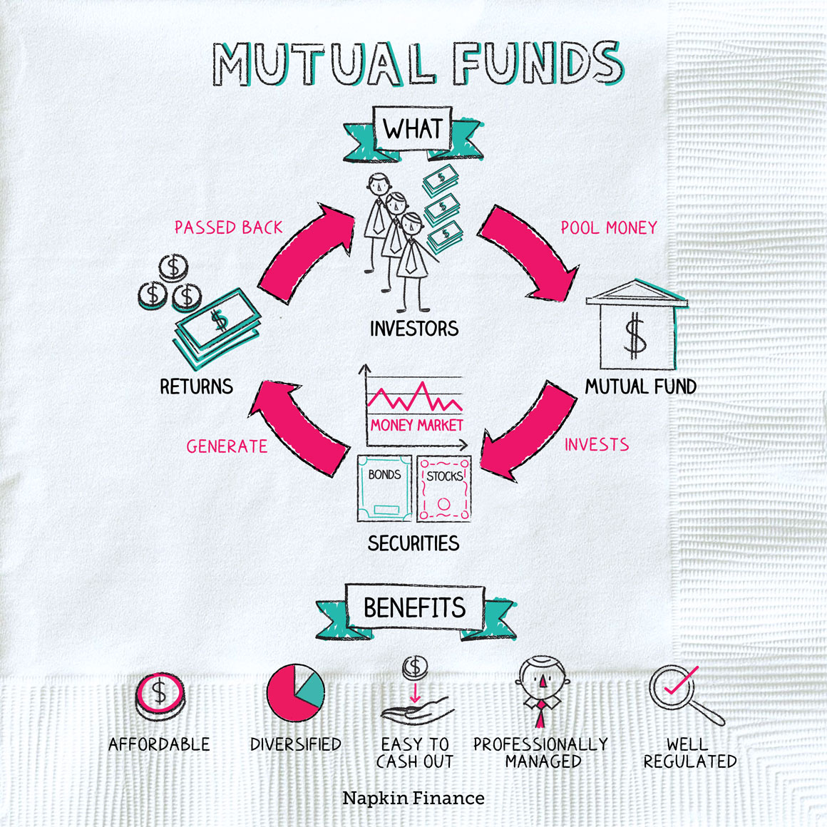
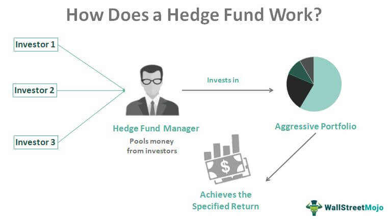
For this reason, many banks and other financial institutions offer investment funds which are managed by professionals. Mutual funds⁵⁶ are one such option which pulling money from multiple investors and then buy shares on their behalf.

You can choose funds according to your investment goals. Some are designed to reduce risk, yield a lower expected rate of return while others are configured to give a higher rate of return at increased risk.

Some funds track the performance of specific sectors such as infrastructure, technology, communications, et cetera while others may be tied to specific indices.

In addition to combining multiple stocks, some funds are traded on stock exchanges themselves.

That is, in order to invest money in these funds, you buy their shares on the market.

Hence, they are known as Exchange Traded Funds or ETFs.

They are very popular investments for stock market investors as it tend to produce ome growth as long as the sector or index they’re tracking does well. In addition to mitigating risk, they are also much more economically compared to investing in many stocks individually, because you typically have to pay brokerage and other transaction fees on them separately.

A popular ETF is Standard & Poor’s 500 or S&P 500 which trades under the ticker symbol SPY. S&P 500 include 500 stocks with the large market capitalization that trade on the New York Stock Exchange or Nasdaq, selected from diverse sectors.

The composition of an ETF, the stocks and their proportions can vary over time. This gives rise to another source of information that can be useful in making trading decisions.

Stock Returns

Returns

What we care about is how our investment has increased or decreased in value. So, how do we measure that increase or decrease?

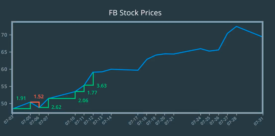
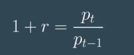
There are actually several metrics we might use to quantify changes in price over time. One is the simple difference in price. \(P{_t}-P_{t-1}\)

This might represent the difference between the price of a stock this month and it’s price one month ago for example.

Another is the percentage return or raw return. This is the difference divided by the starting price, \(\frac{P_{t}-P_{t-1}}{P_{t-1}}\) Imagine you bought a $1,000 of stock one month ago and sold it this month for $1050.

Your return on your initial investment of $50 is five percent of your original investment. If you buy $5,000 of stock this month and sell it for $5,300 next month, you might want to compare the success of this new investment to the previous one. Instead of comparing $300 to $50, you can calculate the return and compare six percent to five percent to see that as a proportion of your original investment.

The raw return may be referred to simply as the return , or alternatively, as the percentage return , linear return , or simple return . It is defined as \(r = \frac{p_t - p_{t-1}}{p_{t-1}}\)

Log Returns

Quantitative analysts frequently work with a quantity related to but slightly different from the raw return, the natural logarithm of return.

Remember how the return was defined as \(r = \frac{p_t - p_{t-1}}{p_{t-1}}\) Well, the log return is defined slightly differently, as the natural logarithm of \(r_{\log} = \log_e({\frac{P_t}{P_{t-1}}}) = \ln({\frac{P_t}{P_{t-1}}})\) if we do: \(\frac{P_t - P_{t-1}}{P_{t-1}} + 1 = \frac{P_t}{P_{t-1}}\)

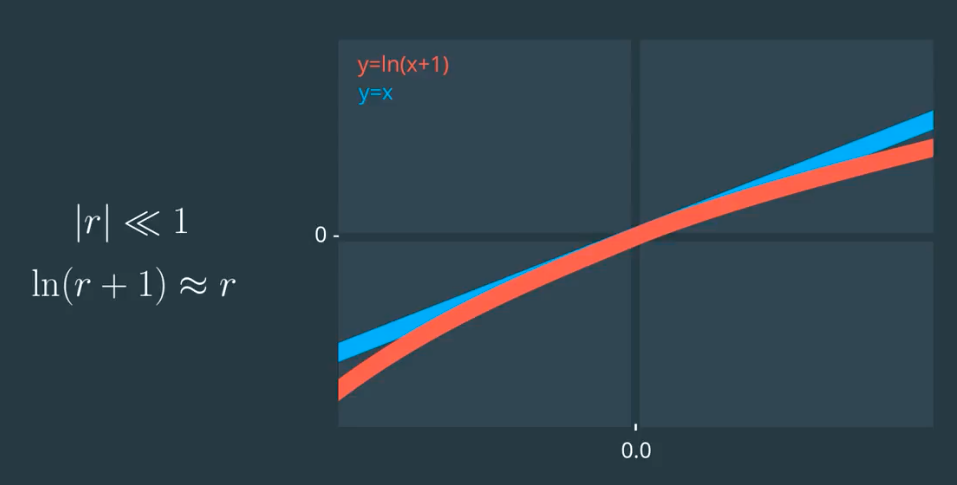\(\text {log return} = R = \ln\left(\frac{p_t}{p_{t-1}}\right) \\ \\ \text {raw return} = r = \frac{p_t - p_{t-1}}{p_{t-1}}\) Converting them: \(R=ln(r+1) \\ \\ r = e^R - 1\)

Log returns and Compounding

Log returns can be convenient for calculations that involve compounding⁵⁷. To explain this idea, let’s first discuss compounding.

The idea of compounding is a simple one. Say you put $100 in a bank account that earns 4% interest per year, compounded annually. After 1 year, you have

$100 + $100*0.04 = $104.

The next year, you have,

$104 + $104*0.04 = $108.16,

so you earned another $4 of interest on the original $100 but also 16 cents on the $4 of interest earned last year.

Compounding is the process by which an asset’s earnings are reinvested to generate additional earnings, that is to say, earning interest on interest.

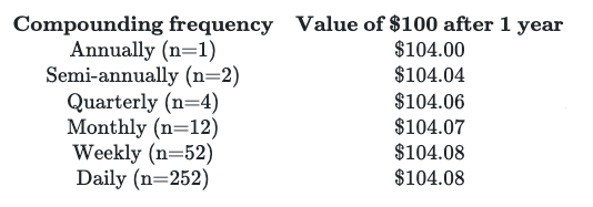
Looking at the table, you can see that with more frequent compounding, the value at 1 year increases but then seems to level off. If you assumed that the benefit of compounding more and more frequently had a limit, you would be right! How do we calculate this limit? Well, first we write down the formula for compounding, \(P_t = P_{t-1}(1+\frac{r}{n})^n\) and then we notice that what we’d like to do is make n bigger and bigger. We want the limit as n goes to infinity. Well, it turns out that this limit is: \(\lim_{n\to\infty}(1+\frac{r}{n})^n = e^r\) Compounding infinitely often is called continuous compounding . So what does this mean? Well, it means that if you wanted to calculate how much money you’d have at the end of the year if you started with $100 and compounded continuously , but at a simple annual rate of 4%, you’d calculate: \($100×e^{.04}=\$104.08\)

You’ll notice that the value after 1 year with continuous compounding is pretty close (it’s the same if we round to two decimal places) to the value after 1 year with daily compounding.

Now, say you were trying to reverse the previous calculation. Say you knew you had $104.08 at the end of the year, and $100 at the beginning of the year, and you wanted to calculate the rate of interest as if it had been compounded continuously . You would simply invert the formula. So you’d calculate: \($104.08/$100=e^r\) Then you’d take the natural log of both sides, and then you’d have, \(\ln($104.08/$100) = r\) So: \(0.04 = r\)

r is the continuously compounded annual return . So the continuously compounded annual return equals $\ln(p_t/p_{t-1})$ . But what is this quantity? It’s just the log return! This is why you might hear log returns called continuously compounded returns .

Now, say we invested $100, and the monthly continuously compounded interest rate was 2%. At the end of the month, we’d have \(\$100 \times \mathrm{e}^{.02} = \$102.02\) But if the investment continued to accrue at a monthly continuously compounded rate of 0.02 for a whole year, we’d have $$ $100×e^ .02 ×e^ .02 ×e^ .02 ×e^ .02 ×e^ .02 ×e^ .02 ×e^ .02 ×e^ .02 ×e^ .02 ×e^ .02 ×e^ .02 ×e^ .02

\(… in total, 12 factors of\)\mathrm{e}^{.02}$$ .

So we’d have \($100×(e^ {.02∗12} )=$127.12\) Equivalently, \($100×e^ .24 =$127.12\) Since the annual rate of continuous compounding, 0.24, is simply the sum of the monthly rates of continuous compounding, we say that the continuously compounded rate of return is additive over time .

So, as you can see, the rate of continuous compounding is additive over time. Since, mathematically, the rate of continuous compounding is just the log return, this means that log returns are additive over time, and this can be very convenient. As another example,

log return for January+log return for February

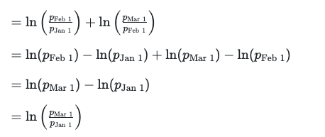
=log return for January and February

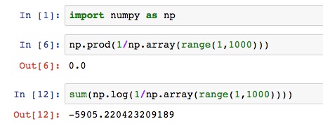
Multiplication of many small numbers can result in the problem that the product is smaller than the smallest number representable in computer memory. Sometimes the computation will incorrectly yield the value 0. This is called arithmetic underflow . The use of logarithms can help with this, since it enables the representation of much smaller (and much larger) numbers. For example:

Distributions of Returns and Prices

Investors are always interested in the potential appreciation⁵⁸ or depreciation⁵⁹ of financial assets. They’d like to be able to predict what will happen to assets in the future, hence, they’d like to be able to build models of stock prices and returns.

An important first step is to think of these prices and returns as random variables , i.e. outcomes of random phenomena, that take on values as described by distributions .

Distributions allow us to summarize the behavior of random variables. So, what are the distributions of returns and prices?

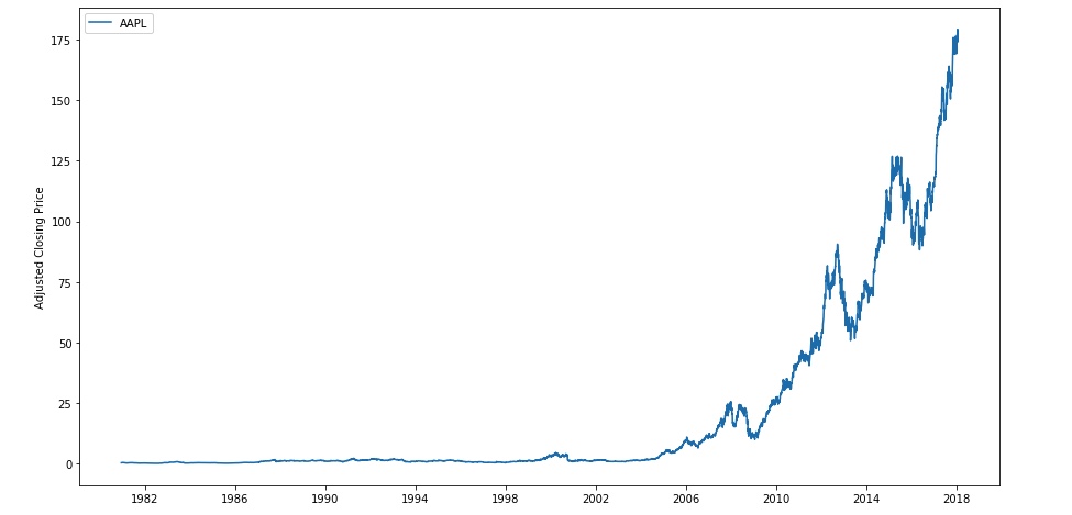
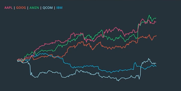
One strategy for getting a sense of potential future behavior is to look to the past. Let’s look at some data from the stock of a familiar company with a storied past, Apple Inc.

Let’s look at the adjusted closing price of Apple stock (AAPL) from 1980 up until the present.

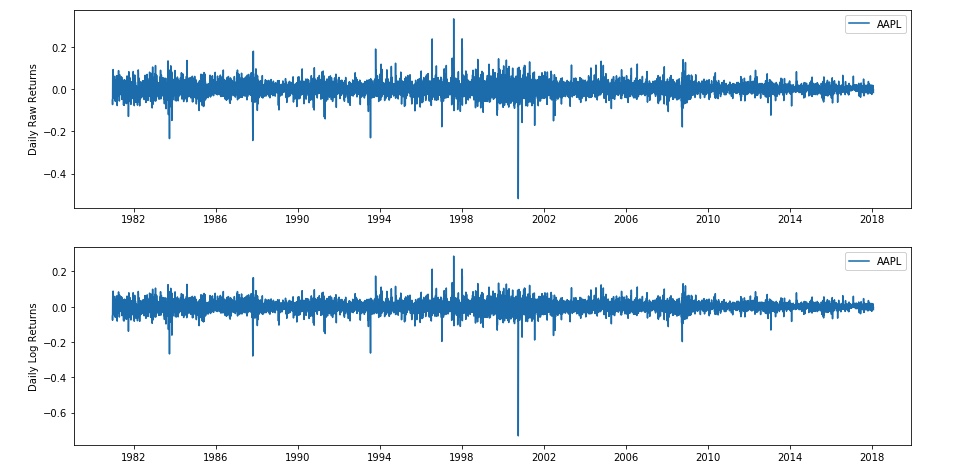
If we calculate returns and log returns on these data and plot them, we’ll see something like the graphs below.

These plot look almost the same—that’s because the returns and log returns for these daily data have very similar values . This is because daily returns are small—the values are close to 0, so the property $\ln(1 + r) \approx r$ applies. But we’re interested in the distribution of these values, so let’s look at a histogram.

Here we’ve plotted a histogram of AAPL’s log returns from 1980 to the present, and we’ve overlaid a scaled normal distribution. We can see a few things right away from this plot. First, the values are centered around 0, and in fact look roughly normal. However, the tails of the histogram clearly lie above the tails of the normal distribution. We call these “fat tails”.

In general, the normal distribution can be a reasonable approximation for short-term returns and log returns for some applications. However, many analyses have shown that the data do not conform perfectly to a normal distribution, and often deviate significantly in the tails. The significance of this is that the normal distribution predicts fewer extreme events than are actually observed. The conversation about the best model for the distribution of returns has been going on for at least the past century. The best model will depend on exactly what your analysis seeks to achieve.

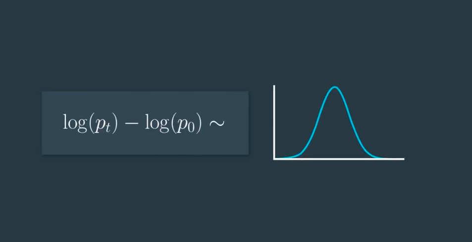
Based on historical data, it may be reasonable to consider short-term returns as approximately normally distributed for some purposes. However, even if short-term returns are normally distributed, long-term returns cannot be. If $r_1 = \frac{p_1 - p_0}{p_0}$ and $r_2 = \frac{p_2 - p_1}{p_1}$ are normally distributed, the sum of these, $r_1 + r_2$would be normally distributed. But the two-period return is not the sum of the one-period returns.

Two-period return

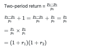
The product$ (1 + r_1)(1 + r_2)$ is not normal, and becomes noticeably less normal as the product grows over time.

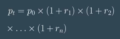
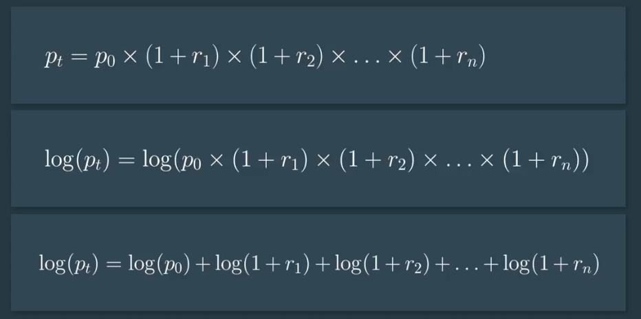
Let’s talk about how a series of daily price values arises. It has to do with our earlier discussion of compounding. Let’s say, a stock starts at P sub zero, (P_0) and each day the price changes by some small percent, the return. (r).

We saw earlier how the price at time T could be written as a product of all of these one plus little r sub i terms.

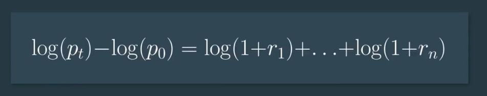
If we take the log of both sides of this equation,

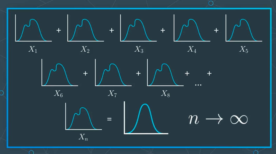
Now, we’re going to use the central limit theorem.

It says that, the sum of random variables that have the same distribution and are not dependent on each other approaches a normal distribution and the limit that the number of random variables and the sum goes to infinity.

So, let’s make the assumption that the returns on each day are independent, but come from the same underlying distribution.

This seems reasonable certainly more reasonable for returns and for prices. After all, the price of a stock on one day almost certainly depends on its price the day before.

So, if we make that assumption,

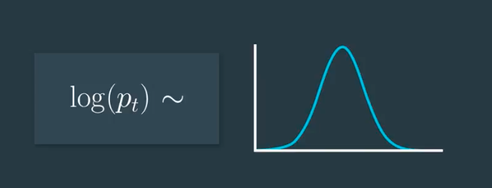
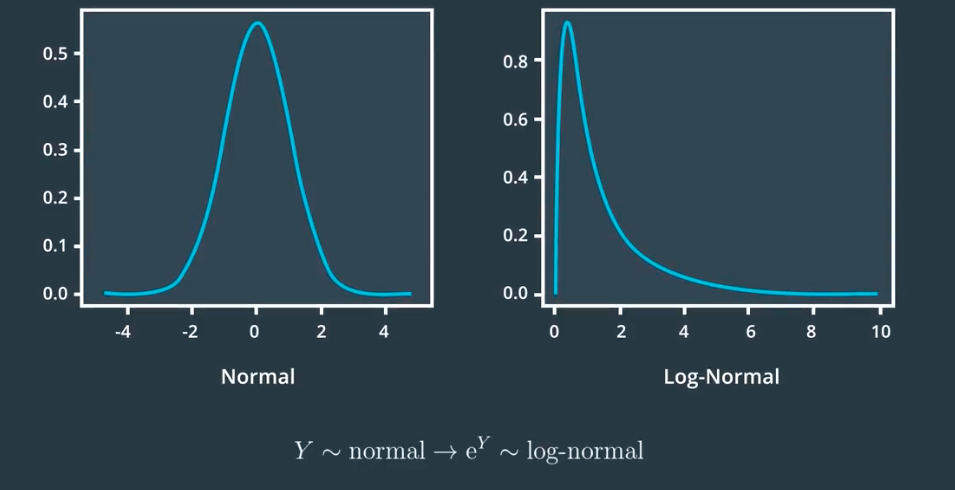
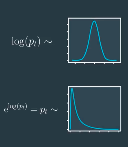
However, when working with real data, the assumption that prices are distributed log normally, may or may not be a good one. These distributions can be convenient models, but don’t confuse them with actual distributions of stock prices or returns.

So long-term prices and cumulative returns can be modeled as approximately lognormally distributed because they are products of independently, identically distributed (IID) random variables.

On the other hand, log returns sum over time.

Therefore, if $R_1 = \ln\left(\frac{p_1}{p_0}\right)$ and $R_2 = \ln\left(\frac{p_2}{p_1}\right)$are normal, their sum, the two-period log return, is also normal. Even if they are not normal, as long as they are IID, their long-term sum will be approximately normal, thanks to the Central Limit Theorem. This is one reason why using log returns can be convenient for modeling purposes.

1. Log returns can be interpreted as continuously compounded returns.
2. Log returns are time-additive. The multi-period log return is simply the sum of single period log returns.
3. The use of log returns prevents security prices from becoming negative in models of security returns.
4. For many purposes, log returns of a security can be reasonably modeled as distributed according to a normal distribution.
5. When returns and log returns are small (their absolute values are much less than 1), their values are approximately equal.
6. Logarithms can help make an algorithm more numerically stable.

Momentum Trading

Designing a Trading Strategy

A trading strategy is a set of steps and rules that help you decide what stocks to buy or sell, when to perform these trades and how much money to invest in them.

In order to have a competitive advantage over other traders, you should try and come up with your own ideas or variations.

Momentum Based Signals

Newton’s first law of motion states that an object at rest stays at rest, and an object in motion stays in motion with the same speed and in the same direction, unless acted upon by an unbalanced force.

While Newton’s laws may seem to have little to do with the vagaries of the stock market, a similar behavior is often noted in security prices, that is, rising stock prices seem to continue to rise for some time, while falling stock prices continue to fall.

This observed phenomenon is popularly known as momentum⁶⁰.

But, stocks are not like physical objects, so what causes this effect?

There are several factors that seem to contribute to it including human behavior. People don’t want to miss out on an opportunity to make money, and tend to follow the heart. People also tend to under-react to news. New information propagates over time leading to a prolonged effect on stock prices.

There is a branch of trading strategies that attempts to capitalize on such trends, and while there is no standard method to quantify momentum signals, a few common techniques include: technical indicators such as moving averages, large price movements with volume, and stocks making new highs.

The general premise of this trading signal is that, out-performing stocks tend to keep their momentum and continue to remain out-performers for some more time in a particular market and vice versa for under-performers.

If you believe in momentum being a repeating market phenomenon, it may be a good opportunity to buy out performers and sell under-performers, capitalizing on the continuation of their movement.

Long and Short Positions

Once you have found a signal that seems to indicate the future performance of a stock, it is time to put it to action.

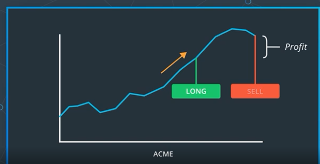
For instance, if you think that a stock has upward momentum, you might want to buy some shares and hold onto it for a fixed period of time, or until you start seeing the stock fall. This is known as taking a long position on the stock.

When you sell your stock, hopefully, at a higher price than you bought it, that is known as closing your position.

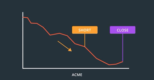
It might sound bewildering⁶¹. But what it boils down⁶² to is borrowing shares from someone, usually your broker, and then promising to return them once your short position is closed.

The brokers incentive⁶³ here is that they typically earn a commission on the profit you make from the short sale.

At the same time, they are taking a risk. What if you bail out⁶⁴ and never buy back the shares?

For this reason, brokers typically require you to keep some money in a margin account that they can charge if you fail to keep your promise. The whole process of short selling is a bit more complex with interests⁶⁵, fees⁶⁶, and margin calls⁶⁷ coming into the picture.

But, all you need to know when evaluating a potential trading signal is that shorting is one possible action you can take.

So, when you think a stock is going up, you can buy or go long, and if you believe it is going to keep falling, you can short it.

However, dealing with individual stocks can be tricky and unpredictable. You don’t want to put all your eggs in one basket. Therefore, it is recommended to adopt a cross-sectional strategy, where you invest in multiple stocks at the same time.

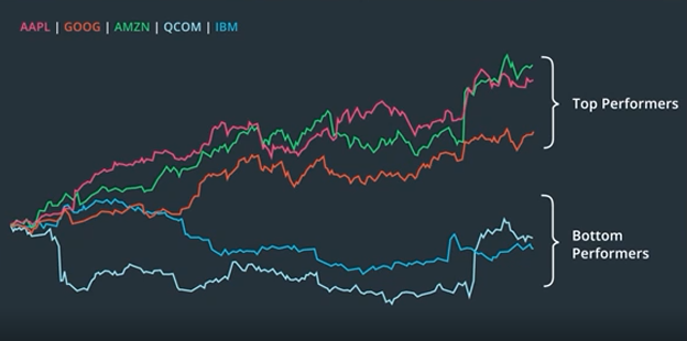
One smart way to do this is to use your signal to rank order the stocks⁶⁸, and use the rankings to select stocks for long and or short positions.

For instance, if you’re using a momentum signal, the top performers are likely to keep rising, so you can go long on them, and the bottom performers, that are falling, are likely to keep falling. So, you can short them.

Portfolio — A portfolio is a collection of investments held and/or managed by an investment company, hedge fund⁶⁹, financial institution or individual.

Long — A long (or long position) is the purchase of an asset under the expectation that the price of the asset will rise.

Short — A short (or short position) is the selling of an asset under the expectation that the price of the asset will decline. In practice, an investor profits from a short position by borrowing shares from a brokerage firm (agreeing to pay an interest rate as a fee), selling them on the open market, and later buying them back on the open market at a lower price and returning them to the brokerage firm.

Trading Strategy

Statistical Analysis

Now we are ready to perform our analysis. The resulting returns time series⁷⁰ is the theoretical monthly performance of our long-short portfolio.

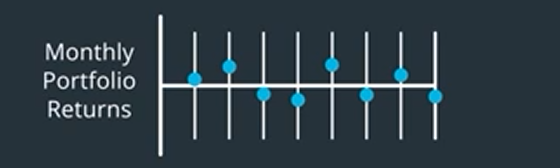
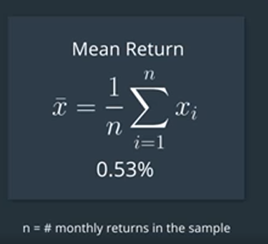
Our goal is to see if the mean monthly return is greater than zero. Let’s calculate that.

On average this trading strategy yields positive returns? That is to say that the true mean is greater than zero? It could be that on average this trading strategy will not yield positive returns.

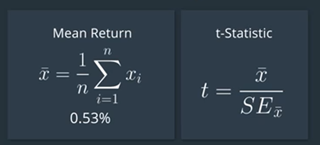
Maybe the true mean is less than or equal to zero, and this value is just a random fluctuation⁷¹.

Well, one approach to assess this is to perform a statistical test on our hypothesis. A t-test is a way of testing the probability of getting as bigger mean as we did, assuming all the assumptions we made to build our model of strategy returns were correct.

Using this t-statistic, we can measure the probability of getting a mean monthly return of 0.53 percent or larger if the true mean monthly return is zero given that the assumptions we made to build our model are correct.

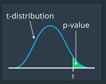
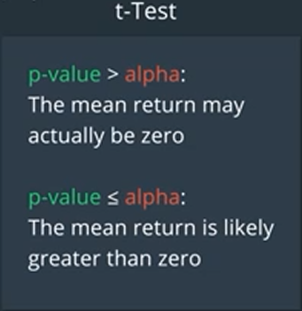
This probability is called the p-value. If the probability is very small, we might infer that it’s unlikely that the true mean is zero.

Now, before running the test, we should decide how small the p-value needs to be for us to conclude that the true mean is not zero.

To denote this threshold, we usually use the Greek symbol alpha. A commonly used value is 0.1.

The Many Meanings of “Alpha”

The term “alpha” is used to mean multiple things in the investment industry.

In mathematics, you’ll see alpha refer to the significance level of a hypothesis test. In regression, you’ll see alpha refer to the y-intercept of a straight line.

In finance, alpha refers to multiple distinct but somewhat related ideas. The common thread among these definitions is that alpha is the extra value that an investment professional can add to the performance of an investment.

One specific definition of alpha is the extra return that an actively managed fund can deliver, that exceeds the performance of passively investing (buy and hold) in a portfolio of stocks. Another specific definition of alpha, which we’ll primarily focus on in this course, is that of an alpha vector.

An alpha vector is a list of numbers, one for each stock in a portfolio, that gives us a signal as to the relative future performance of these stocks. You’ll learn more about alpha vectors throughout term 1.

Just to be clear, the finance community, both in academia and industry, use alpha to denote multiple ideas.

Finding Alpha

Formulating trading strategies often starts with an observation. A pattern that seems to be recurring in the market over time. At that point, your creativity and intuition tell you that there might be an opportunity for monetization.

Your job as a quant trader then, is to turn this observation into an expression, both mathematically and programmatically and verify it using historical data. This is alpha research.

Statistical analysis lets you very quickly and scientifically test whether an observed pattern or trading signal that you come up with has the potential to turn into a profitable trading strategy. Once this is proven, then you can proceed to define your trading strategy in a more detailed manner. Which will lead to a full back-testing exercise, as the last step of the research process.

P1 — Trade with Momentum

Mindmap and Assets

Quant Basics
	Stock Prices
	Market Mechanics
	Data Processing
	Stock Returns
	Momentum Trading

Advanced Quants
	Quant Workflow
	Outliers and Filtering
	Regression
	Time Series Modeling
	Volatility
	Pairs Trading and Mean Reversion
	Breakout Strategy [P]

Funds, ETFs, Portfolio Optimization
	Stocks, Indices, Funds
	ETFs
	Portfolio Risk and Return
	Portfolio Optimization
	Smart Beta and Portfolio Optimization [P]

Factor Investing and Alpha Research
	Factors
	Factor Models and Types of Factors
	Risk Factor Models
	Time Series and Cross Sectional Risk Models
	Risk Factor Models with PCA
	Alpha Factors
	Alpha Factor Research Methods
	Advanced Portfolio Optimization
	Alpha Research and Factor Modeling [P]

Quant Basics
	Stock Prices
	Market Mechanics
	Data Processing
	Stock Returns
	Momentum Trading

Advanced Quants
	Quant Workflow
	Outliers and Filtering
	Regression
	Time Series Modeling
	Volatility
	Pairs Trading and Mean Reversion
	Breakout Strategy [P]

Funds, ETFs, Portfolio Optimization
	Stocks, Indices, Funds
	ETFs
	Portfolio Risk and Return
	Portfolio Optimization
	Smart Beta and Portfolio Optimization [P]

Factor Investing and Alpha Research
	Factors
	Factor Models and Types of Factors
	Risk Factor Models
	Time Series and Cross Sectional Risk Models
	Risk Factor Models with PCA
	Alpha Factors
	Alpha Factor Research Methods
	Advanced Portfolio Optimization
	Alpha Research and Factor Modeling [P]